and the distribution of digital products.
Recasting Three-Peak Exclusion Limits on B − L Dark Matter via Accelerometer Studies
:::info Authors:
(1) Dorian W. P. Amaral, Department of Physics and Astronomy, Rice University and These authors contributed approximately equally to this work;
(2) Mudit Jain, Department of Physics and Astronomy, Rice University, Theoretical Particle Physics and Cosmology, King’s College London and These authors contributed approximately equally to this work;
(3) Mustafa A. Amin, Department of Physics and Astronomy, Rice University;
(4) Christopher Tunnell, Department of Physics and Astronomy, Rice University.
:::
Table of Links2 Calculating the Stochastic Wave Vector Dark Matter Signal
3 Statistical Analysis and 3.1 Signal Likelihood
4 Application to Accelerometer Studies
4.1 Recasting Generalised Limits onto B − L Dark Matter
6 Conclusions, Acknowledgments, and References
\ A Equipartition between Longitudinal and Transverse Modes
B Derivation of Marginal Likelihood with Stochastic Field Amplitude
D The Case of the Gradient of a Scalar
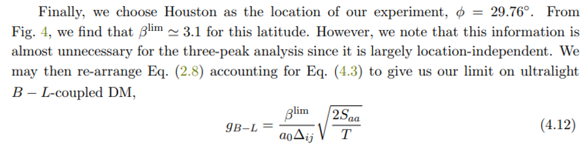
4.1 Recasting Generalised Limits onto B − L Dark MatterTo recast our limits on β shown in Fig. 4 into one on the parameter of interest for this model, the gauge coupling strength gB−L, we must define four quantities. Firstly, we must make clear what the quantity A is for this experiment, which will depend on both the model and the signal of interest for this sensor. Secondly, we must choose an observation time, Tobs. Thirdly, we must elaborate on what the concrete noise profile, σ(ω), for this type of experiment is. Lastly, and least importantly following from our discussion above, we must choose a latitude for the experiment. Once these are known, Eq. (2.8) can be re-arranged for gB−L, giving us our model- and experiment-specific 90% CL limit.
\ For B − L coupled dark photon dark matter, the relevant signal is a differential acceleration. This is given by Eq. (2.6) in the time domain, with a now concrete choice for A,
\
\

\ Here, gB−L is the gauge coupling strength of the model, ∆ij is the differential B −L charge per nucleon between materials i and j, given by
\
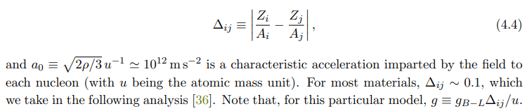
\ For our observation time, we take Tobs = 10T⊕ to be firmly in the regime where the three peaks can be resolved. For light cavities, which may only be able to remain coherent over the scale of hours rather than days, such a runtime is optimistic. However, since our aim here is merely to showcase how our method can be used concretely and compare to the works of Refs. [36, 38], we do not see this as an issue. Our strategy is general and can be applied to any axial sensor and vector-like DM model, and we have settled on this configuration only for the sake of argument; other sensor technologies, such a magnetically levitated sensors, do not have this issue. Moreover, multiple cavities or data-stacking techniques can be employed to mitigate this issue.
\
\
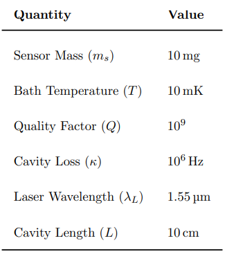
\ Our choices for all of the above parameters except for the laser power, which we expand on below, are summarised in Table 1. These are in keeping with the choices made in Refs. [36, 38].
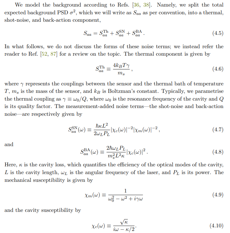
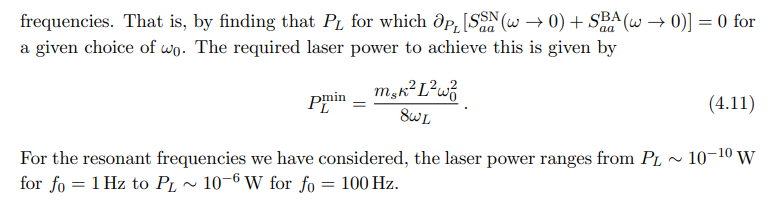
\ The choice of where to tune the laser power is critical to give us competitive limits for a wide range of dark matter masses. We have found that we can achieve excellent limits for low dark matter masses, which are of most relevance to our work, by tuning the laser power such that the back-action and shot-noise components are minimised at low
\
\
\
\ We note that this choice of power tuning is different from the strategies usually employed in other studies. Typically, the laser power is tuned so that the measurement-added noise is either minimised on resonance or, as LIGO implements it, well above resonance [88]. However, we found that both of these choices detriments the limit that we can draw at low masses, increasing the background at low frequencies beyond the thermal noise floor. For these other strategies to be beneficial at both the respective frequency targets and at low frequencies, the thermal noise would have to be significantly lower than that achieved with our choice of sensor mass, quality factor, and bath temperature.
\ In the treatment of our backgrounds, we have neglected seismic noise, which can become important at frequencies below ∼ 10 Hz. Since we require the use of two materials to measure the differential acceleration peculiar to B − L DM, we can envision constructing two sensors: one with a moveable mirror made of material i and another of material j. By subtracting their signals, we both isolate the differential acceleration signature and remove backgrounds common to both—this includes the seismic noise component [63]
\
\
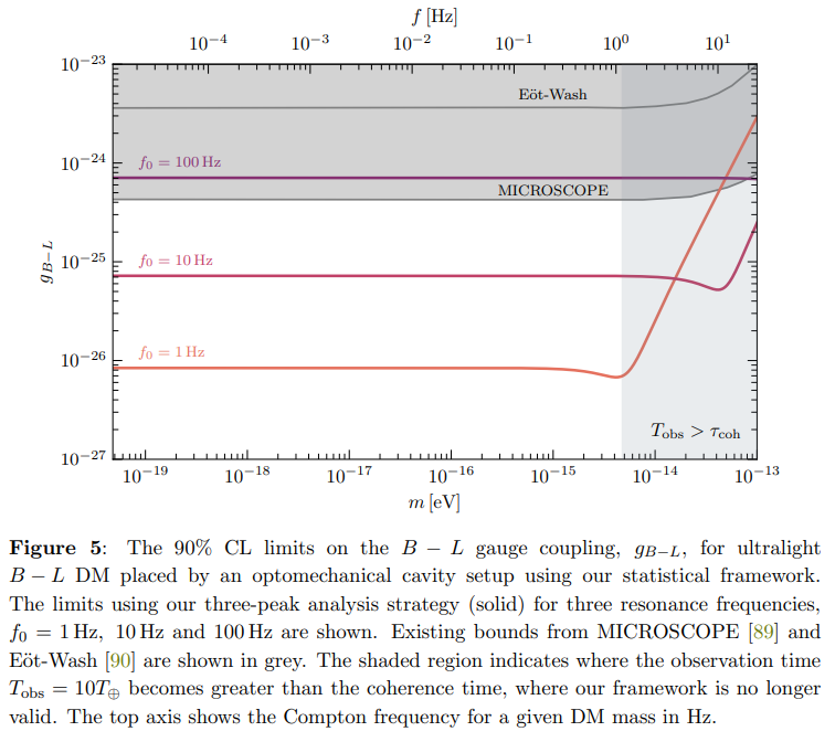
\ We show our limits in Fig. 5 for three choices of resonance frequency: 1 Hz, 10 Hz and 100 Hz. For all but the last of these frequencies, we are able to exclude new regions of the UDLM B − L parameter space, best excluded by the fifth-force satellite experiment MICROSCOPE [89] and torsion-balance experiment E¨ot-Wash [90]. This showcases the power of such sensors in searching for this DM candidate, as was first pointed out in Ref. [63]. In a single-peak analysis focusing solely on the Compton peak, our limits would be weakened by approximately a factor of 2, as can be seen from Fig. 4. This difference becomes more dramatic for sensors located closer to the equator.
\
\
\ We note that σ(ω), though mostly slowly varying in the frequency width ∆ω = ω⊕, does exhibit a large gradient around the resonance frequency of the cavity. In the neighbourhood of this frequency, our assumption that σ(ω) does not vary greatly in the above range is incorrect, and a more careful analysis in which all three peaks take on different noise levels would have to be conducted for more representative limits. However, we do not expect that our limits would differ greatly from our calculation and, at any rate, would still smoothly join to the regimes on either side of the resonance frequency, where our assumption holds.
\
:::info This paper is available on arxiv under CC BY 4.0 DEED license.
:::
\