Increasing the Sensitivity of A/B Tests

\ \ Suppose we are engaged in online advertising and have developed a new algorithm for ranking advertising banners. We randomly divide the site users into two groups: A and B - for users from group B, a new improved ranking model will be applied. Let the average profit from showing an ad to one user in group B be higher than in group A by +1%. ==Is this significant or just random noise? What about +10%?== To answer these questions, we need a statistical test. Let’s calculate the so-called Z-statistic:

\

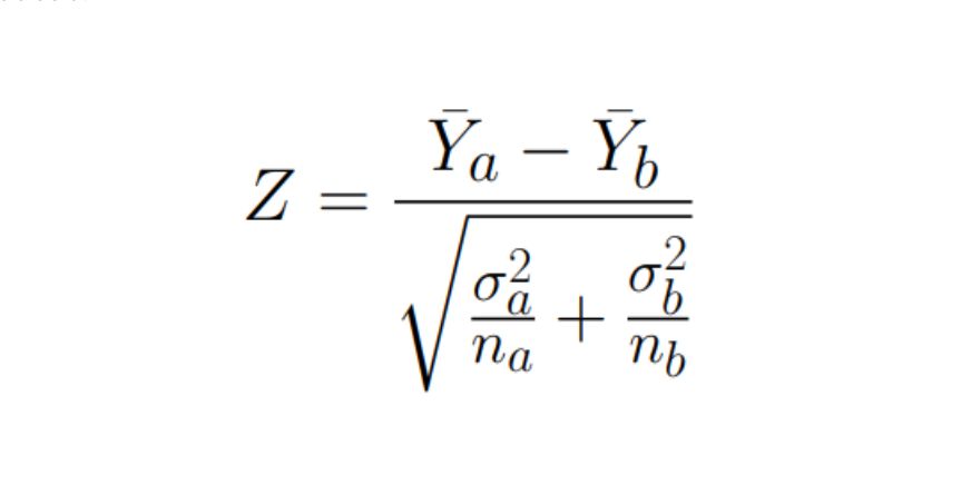
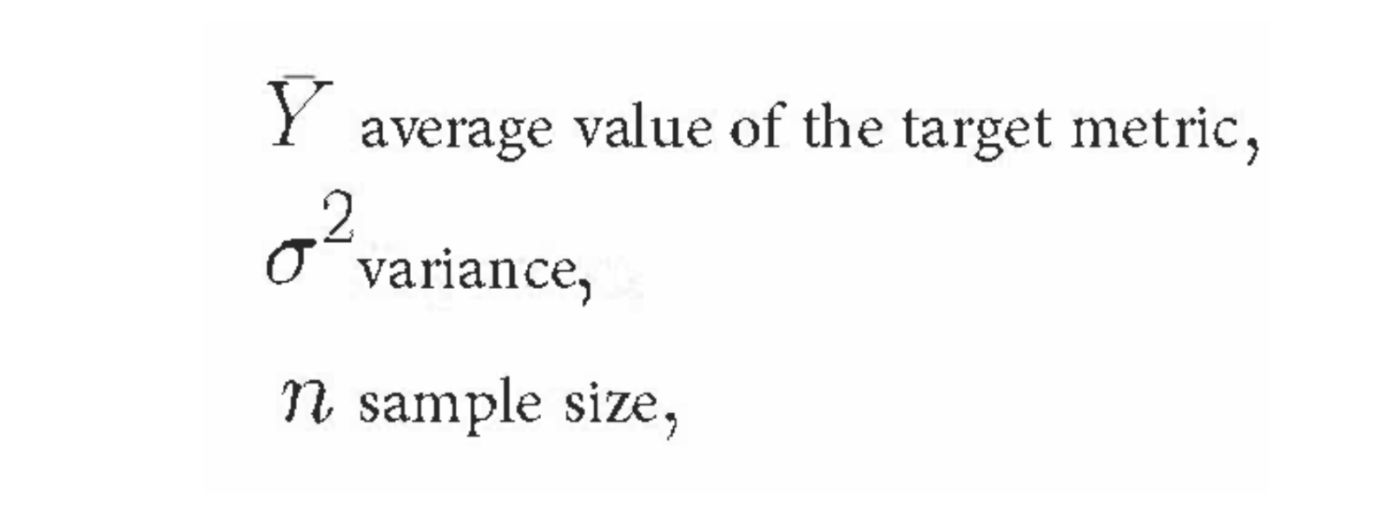
\ where:

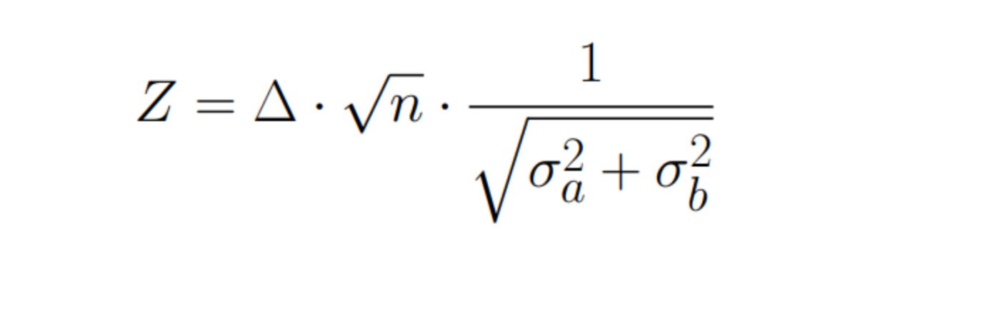
\ Assuming that the sample sizes are equal in groups A and B, let’s rewrite the formula:

\n

If model B does not bring improvement and if the sample size is large enough (usually it is considered that more than 30 is enough), then, according to the central limit theorem, the random variable Z will have a normal distribution:

\n

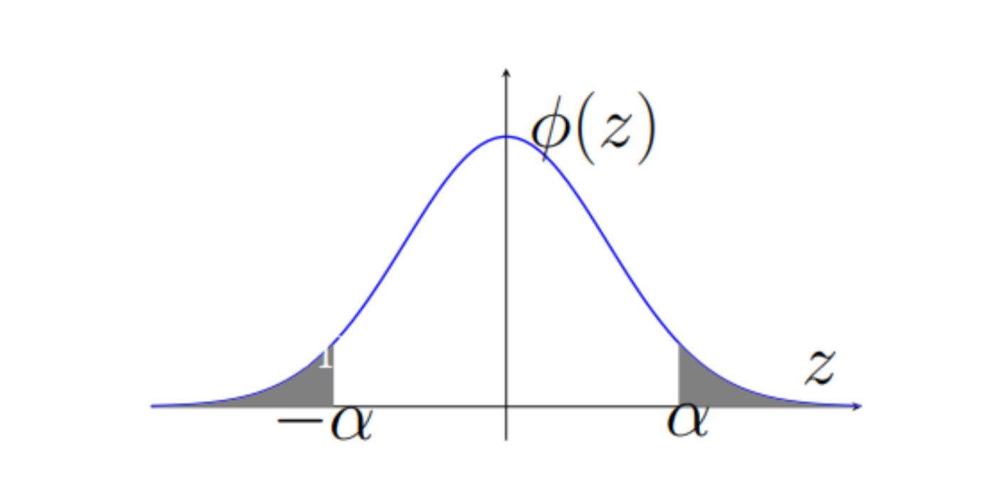
If model B nevertheless brings an improvement (or deterioration), then the distribution of the random value Z will differ from the normal distribution, and the value of the Z-statistic will be far from zero. What value should we consider far from zero? Let's denote it with the letter α and proceed as follows: we calculate the Z statistic; if Z> α, then we conclude that model B is better than model A, and roll it out into production. What is the probability that we would make a mistake?

\ The first option of error - when model B is better than model A, but the value of Z was less than α, and we did not roll anything out. The second option of error - when model B is the same as A, but the value of Z was greater than α, and we rolled out a model that is no better. This second option of error is usually more interesting to us. The probability of making such a mistake is equal to the area of ​​the shaded area in the figure and is called p-value.

\ Now, to find the required α, we set ourselves an acceptable probability of error p-value, that is, we say “with this approach - comparing Z with α we are ready to erroneously roll out model B into production with probability p-value”. Usually, the p-value is chosen around 0.05. That is, we choose such α that the probability of erroneously rolling out the model into production is equal to 0.05. When Z > α, they say that the difference is “statistically significant”.

\ Let’s go back to Z now and see what affects its value. First, the larger the difference between the mean values ​​of the metric for two models (denoted as ∆), the larger Z. This means that if model B is on average much better than model A, then most likely Z will also be greater than α and we will roll out a new model.

\ Secondly, the sample size n affects the value of Z: the larger the sample size, the larger the value of Z. It means that even if the difference between two models is small, by increasing sample sizes we can still make this difference statistically significant and therefore roll out a new model.

\ Sample size is what we can influence as experimenters. But this means either increasing the share of users - participants in an experiment, which can be risky, or increasing experiment time, which is always undesirable and slows down decision making. Moreover, dependence on sample size looks like:

For example, all other things being equal, if in one experiment difference between means of two models was ∆1, sample size n1 and this difference was statistically significant then if in another experiment difference between averages ∆2 = ∆1/2, then to make this difference also statistically significant we need to take n2 = n1 × 4 users. That is, in order to maintain statistical significance, the number of users needs to grow quadratically (!) with the decrease in the difference between the means.

\ Thirdly, the value of Z depends on the following variances:

\

By reducing these variances, we can achieve stat significance.

\ CUPED Method

\ So, if we don’t want to increase sample size n then it remains to reduce variance:

\

A quick reminder:  letter σ denotes standard deviation which is defined as root from variance:

\n

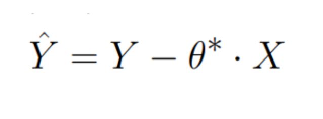
Let’s introduce a new random variable Y which we will calculate as follows (it's going to become clear why very shortly):

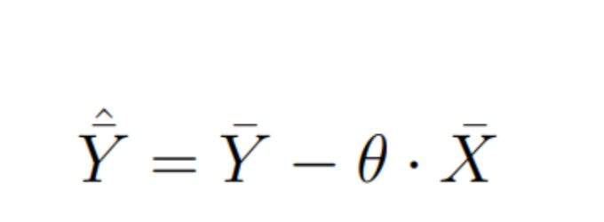
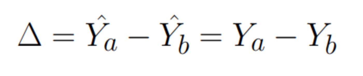
where random variable X does not depend on experiment (a). This condition plays a decisive role. For starters let’s see what would be the delta of our new random variable between samples A and B:

\n

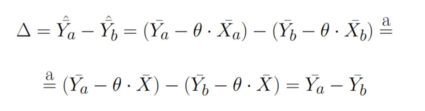
We can omit indices a and b at variables Xa and Xb due to condition (a). Thus, we have proven that the difference of the new random variable between the samples will be the same on average as that of the original random variable Y.. Also, they say that this estimate will be unbiased.

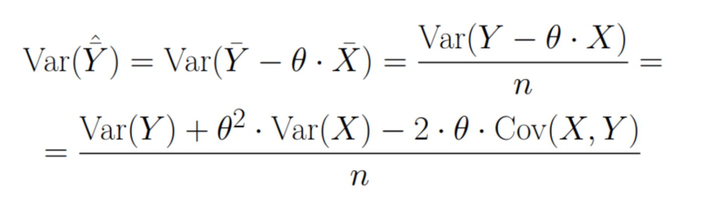
\ It means that we can simply continue calculating our Z-statistic. It remains to understand how variance will change. By definition: \n

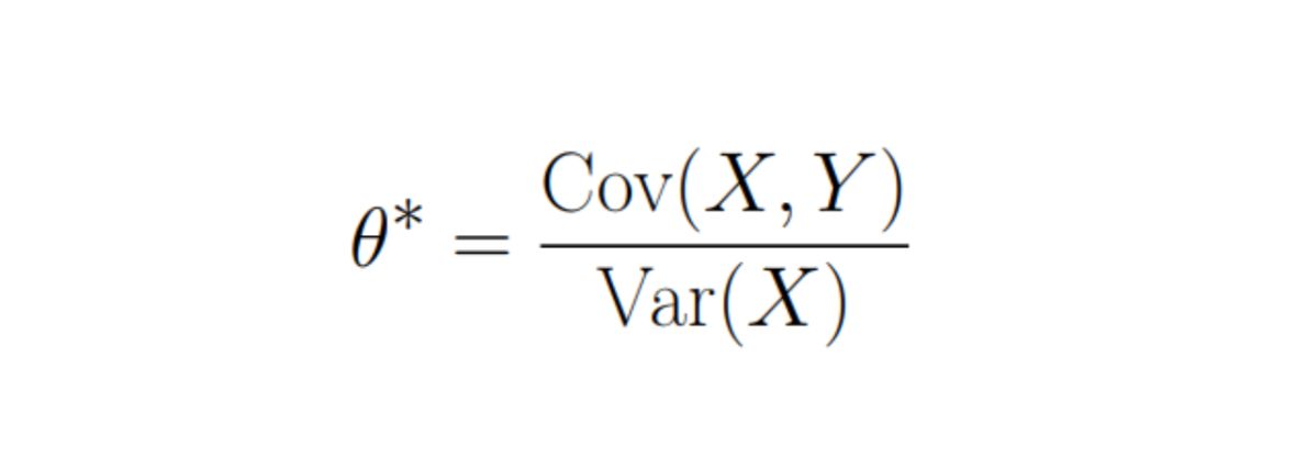
Let’s find where this value is minimal. For this let’s take derivative by parameter θ and equate it to zero: \n

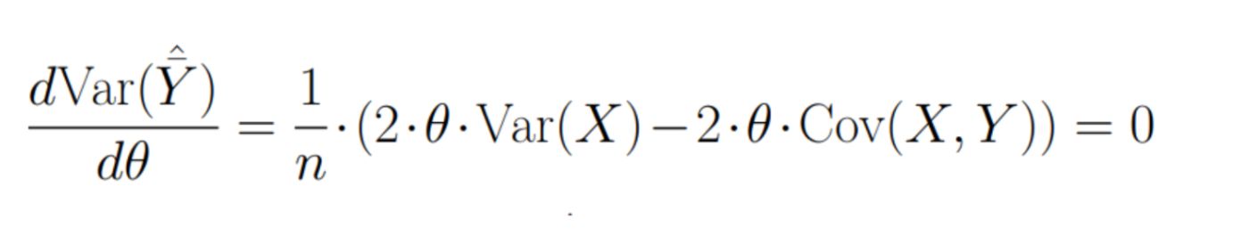
The minimum of Var(Y) is achieved at:

\

And variance value at this point will be equal to (let’s substitute θ* instead of θ): \n

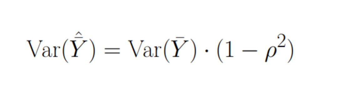
where:

\

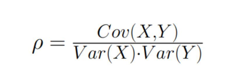
\ \ It is clear that the closer ρ to 1 the smaller (1 − ρ) and therefore smaller variance of the new variable and therefore higher sensitivity of the A/B test!

\ Authors of article Improving the Sensitivity of Online Controlled Experiments by Utilizing Pre-Experiment Data suggest using Y calculated for period before experiment start as X and show that they managed to reduce variance by 50%.

\ What’s next?

\ Let’s take another look at our new random variable:

\

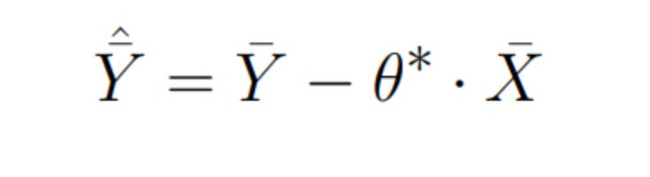
Let’s drop the averaging:

\n

It seems that θ* ·X reminds us of something. Because it is very similar to a  linear model - a feature X and its coefficient θ*. And what if instead of relying on a single coefficient θ* we would train a more complex model F which predicts target variable Y using several features?

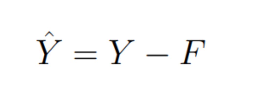
It is important for us that model F does not depend on the experiment in any way:

\n

We can achieve this by building a model on features calculated before starting the experiment.

Let’s look again at what the variance of the new variable will be. By definition: \n

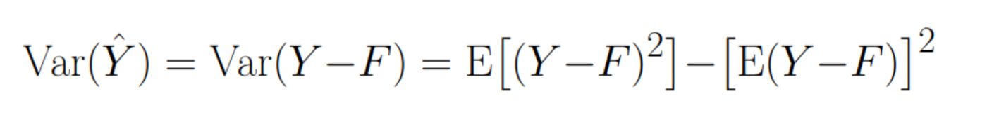
The first term is just a MSE error: \n

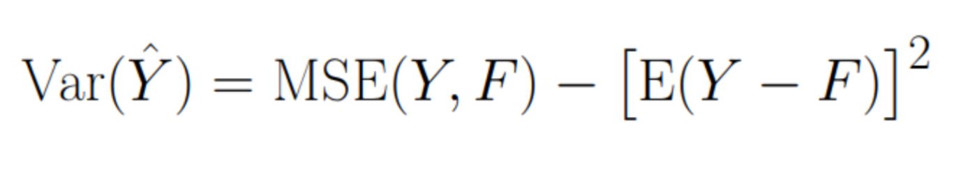
The second term would be equal to 0 if our algorithm gave unbiased estimate of variable Y: \n

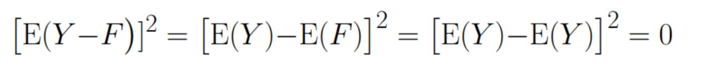
Which model has such conditions? For example, a gradient boosting algorithm with MSE loss  - such a loss function guarantees that the model's prediction will be unbiased.

\ As a result, we get: \n

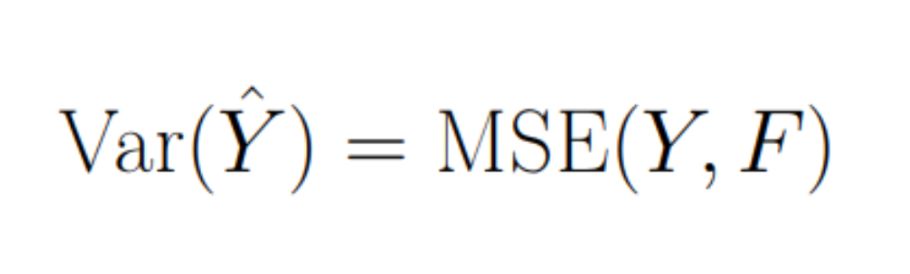
\ That is, the better our model predicts variable Y, the smaller the variance and higher sensitivity of the A/B test will be!

\ This approach was suggested in the article Boosted Decision Tree Regression Adjustment for Variance Reduction in Online Controlled Experiments.