and the distribution of digital products.
What the Phillips Curve Tells Us About Inflation
:::info Author:
(1) David Staines.
:::
Table of Links4 Calvo Framework and 4.1 Household’s Problem
4.3 Household Equilibrium Conditions
4.5 Nominal Equilibrium Conditions
4.6 Real Equilibrium Conditions and 4.7 Shocks
5.2 Persistence and Policy Puzzles
6 Stochastic Equilibrium and 6.1 Ergodic Theory and Random Dynamical Systems
7 General Linearized Phillips Curve
8 Existence Results and 8.1 Main Results
9.2 Algebraic Aspects (I) Singularities and Covers
9.3 Algebraic Aspects (II) Homology
9.4 Algebraic Aspects (III) Schemes
9.5 Wider Economic Interpretations
10 Econometric and Theoretical Implications and 10.1 Identification and Trade-offs
10.4 Microeconomic Interpretation
\ Appendices
A Proof of Theorem 2 and A.1 Proof of Part (i)
B Proofs from Section 4 and B.1 Individual Product Demand (4.2)
B.2 Flexible Price Equilibrium and ZINSS (4.4)
B.4 Cost Minimization (4.6) and (10.4)
C Proofs from Section 5, and C.1 Puzzles, Policy and Persistence
D Stochastic Equilibrium and D.1 Non-Stochastic Equilibrium
D.2 Profits and Long-Run Growth
E Slopes and Eigenvalues and E.1 Slope Coefficients
E.4 Rouche’s Theorem Conditions
F Abstract Algebra and F.1 Homology Groups
F.4 Marginal Costs and Inflation
G Further Keynesian Models and G.1 Taylor Pricing
G.3 Unconventional Policy Settings
H Empirical Robustness and H.1 Parameter Selection
I Additional Evidence and I.1 Other Structural Parameters
I.3 Trend Inflation Volatility
B.5 Consolidation (4.8)Here, I derive the state space form of the non-linear model. The proof uses only techniques from basic analysis. The main complexity arises from the non-linear Phillips curve.
B.5.1 Proof of Proposition 4Proof. Start with the non-linear Phillips curve, formed from substituting the relationship between the optimal relative reset price and inflation derived in Proposition 1 into the left-hand side of (27). Now put (30) and (31) into the right-hand side. Finally, lag the relationship one period to reveal that where W. t are error terms reflecting the difference between expected and true values. They are white noise thanks to the rational expectation hypothesis. Subsequently, dependence on the current shocks will be suppressed. [108]
\

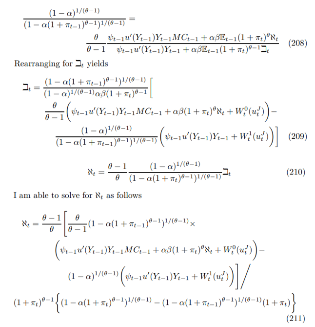
\ where the formula is valid whenever the denominator is non-zero. Now rearranging the future price equation
\

\ then substituting into the right-hand side and simplifying yields
\

\ Moving (207) forward one period and substituting in reveals
\

\

\ To prove this holds with probability one consider
\

\ which appears in the denominator of (207) and (210) through (212), setting the expression equal to zero gives the equation of the singularity
\

\ We can see that this function is surjective, by evaluating its derivative, which shows that it is strictly increasing.
\

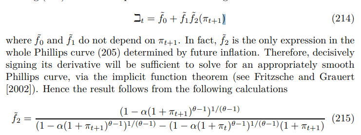
\ This means that the singularity can only occur at a point in time t+1, if inflation is equal to one particular value, determined by inflation in the previous period t. We know this must occur with probability zero as inflation is continuously distributed, since it is determined by the reset price that depends non-trivially on the continuously distributed shock processes.
\ This can be converted into a relationship in expected inflation, by noting that equation (27) and the underlying optimization problems bound inflation above and below as follows
\

\ To complete this section of the derivation all that is required is to substitute out terms in marginal costs and lagged income. Present marginal costs can be removed using (19) and (37) as follows
\

\ leaving only lagged income which can be substituted out via the Euler equation. To this end let us define the following function
\

\ Calling in the policy rule (35), including the output smoothing restriction gives
\

\ which allows us to form a function
\

\ substituting into (217) gives the appropriate form for the Phillips curve
\

\ Finally, we can form the canonical Euler by inverting the Euler using
\

\ then substituting in the Phillips curve gives the final section
\

\ Lastly, by inverting (34), moving one period into the future and substituting in the Phillips curve and noting the expectation must exist to prevent transversality condition blowing again, which means that
\

\
:::info This paper is available on arxiv under CC 4.0 license.
:::
[108] The transversality condition prevents additional non-fundamental terms entering.
\ [109] ZINSS corresponds to a particular case where both singularities arise simultaneously and "cancel out" from the right hand side of (205). The nature of the cocycle at the singularity is treated in the next section.
- Home
- About Us
- Write For Us / Submit Content
- Advertising And Affiliates
- Feeds And Syndication
- Contact Us
- Login
- Privacy
All Rights Reserved. Copyright , Central Coast Communications, Inc.