and the distribution of digital products.
DM Television
Understanding the Phillips Curve: How Economic Trends Shape Inflation and Growth
:::info Author:
(1) David Staines.
:::
Table of Links4 Calvo Framework and 4.1 Household’s Problem
4.3 Household Equilibrium Conditions
4.5 Nominal Equilibrium Conditions
4.6 Real Equilibrium Conditions and 4.7 Shocks
5.2 Persistence and Policy Puzzles
6 Stochastic Equilibrium and 6.1 Ergodic Theory and Random Dynamical Systems
7 General Linearized Phillips Curve
8 Existence Results and 8.1 Main Results
9.2 Algebraic Aspects (I) Singularities and Covers
9.3 Algebraic Aspects (II) Homology
9.4 Algebraic Aspects (III) Schemes
9.5 Wider Economic Interpretations
10 Econometric and Theoretical Implications and 10.1 Identification and Trade-offs
10.4 Microeconomic Interpretation
\ Appendices
A Proof of Theorem 2 and A.1 Proof of Part (i)
B Proofs from Section 4 and B.1 Individual Product Demand (4.2)
B.2 Flexible Price Equilibrium and ZINSS (4.4)
B.4 Cost Minimization (4.6) and (10.4)
C Proofs from Section 5, and C.1 Puzzles, Policy and Persistence
D Stochastic Equilibrium and D.1 Non-Stochastic Equilibrium
D.2 Profits and Long-Run Growth
E Slopes and Eigenvalues and E.1 Slope Coefficients
E.4 Rouche’s Theorem Conditions
F Abstract Algebra and F.1 Homology Groups
F.4 Marginal Costs and Inflation
G Further Keynesian Models and G.1 Taylor Pricing
G.3 Unconventional Policy Settings
H Empirical Robustness and H.1 Parameter Selection
I Additional Evidence and I.1 Other Structural Parameters
I.3 Trend Inflation Volatility
7.1 Slope CoefficientsThe first subsection has the derivation and the second houses the main results.
7.1.1 DerivationIt is most convenient to start with (30) and (31) then apply Theorem 4 from Coayla-Teran et al. [2007], appropriate for (convergent) infinite horizon trajectories
\
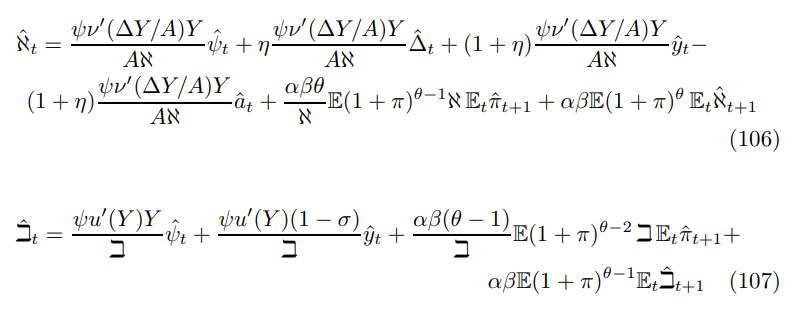
\ where I have used the following substitution derived from (19) and (31)
\
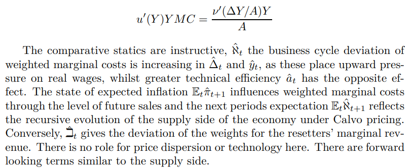
\ The effect of changes in output on marginal revenues depends on the propensity for inter-temporal substitution reflected by σ (the inverse of the elasticity of substitution.) If σ > 1 the propensity to smooth consumption dominates the incentive to substitution over time, such that higher output today implies higher expected future marginal revenues- conversely, if σ < 1 the substitution exceeds the smoothing incentive so higher current output is associated with lower future marginal revenues. When σ = 1 the two forces balance out. Appendix D presents an intuitive argument for σ = 1 valid for this benchmark formulation.
\
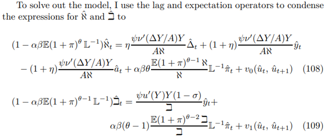
\ The error terms above reflect the difference between the actual and expected values of π, ℵ and i in period t + 1 that comes about because the future value of the structural jump errors are unknown and the model is linear in percentage deviation form. Now using the reset price equation to remove ℵ and i, the price level construction equation to express the reset price in terms of inflation and then manipulating terms in the lag operator yields
\
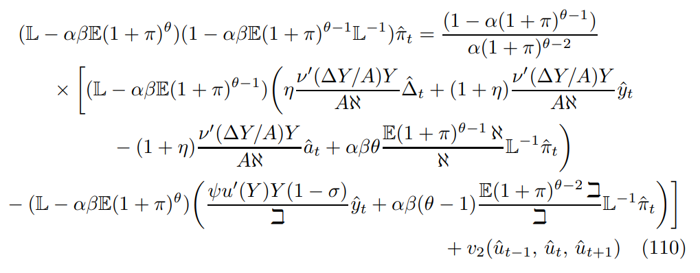
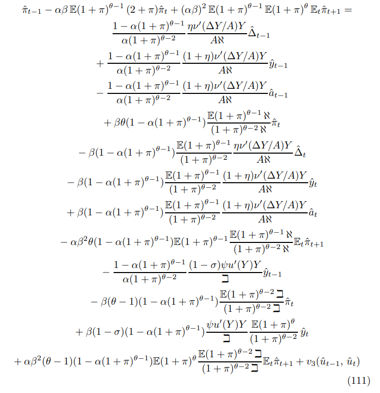
\ Expanding the lag operator, collecting terms and passing expectations from time t yields
\
\

\
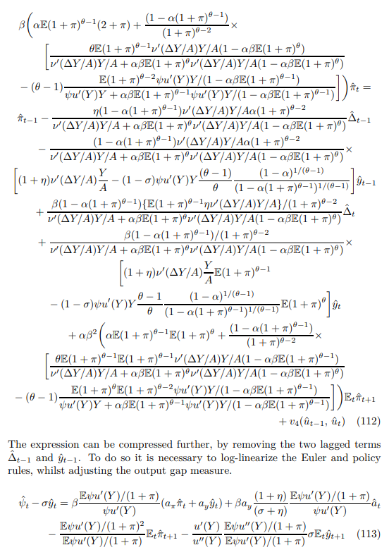
\ Lagging the relationship and including the later period error term yields
\

\ Finally, the log-linearized price dispersion relationship and its lagged form are respectively where I have used the expression for the stochastic steady of ∆
\
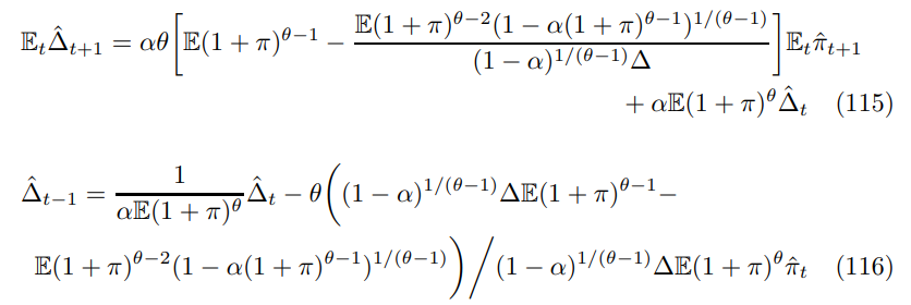
\ Combining (112), (114) and (116) yields the expression for the Phillips curve equivalent to (2)
\

\ By substituting the Phillips curve into the Euler, we have
\

\ For the price dispersion recursion we have
\

\ These are sufficient to describe the canonical form.
7.1.2 Econometrics and ErrorsThis part briefly discusses useful forms for econometric investigation, their basic properties and challenges.
\ It is possible to remove price dispersion as follows[56]
\

\ After taking lags and expanding some expectations, this forms the following Vector Autoregressive Moving Average (VARMA) (p, q)
\
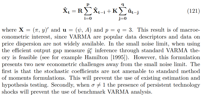
\ The first problem is a long term opportunity for econometrics and mathematical statistics. The second is a more pressing economic concern. It would arise in the benchmark model if one allowed for persistent Euler disturbances. Truncation strategies have been popular (see Ascari and Sbordone [2014]) but there may be scope for refinement.
7.1.3 Slope Coefficients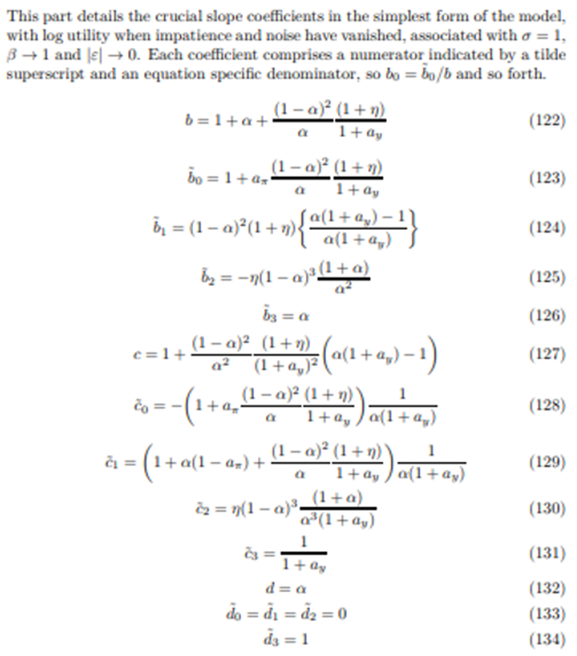
\ Some of these expressions will be discussed and interpreted further in Section 10.
\
:::info This paper is available on arxiv under CC 4.0 license.
:::

- Home
- About Us
- Write For Us / Submit Content
- Advertising And Affiliates
- Feeds And Syndication
- Contact Us
- Login
- Privacy
All Rights Reserved. Copyright , Central Coast Communications, Inc.