and the distribution of digital products.
SALSA Method Applied to Photocatalytic Water-splitting
:::info (1) Sean M. Stafford, Department of Chemical Engineering and Materials Science, Michigan State University, East Lansing, MI, 48824, USA;
(2) Alexander Aduenko, Moscow Institute of Physics and Technology, Moscow, Russia;
(3) Marcus Djokic, Department of Chemical Engineering and Materials Science, Michigan State University, East Lansing, MI, 48824, USA;
(4) Yu-Hsiu Lin, Department of Chemical Engineering and Materials Science, Michigan State University, East Lansing, MI, 48824, USA;
(5) Jose L. Mendoza-Cortes, Department of Chemical Engineering and Materials Science, Michigan State University, East Lansing, MI, 48824, USA (Email: [email protected]).
:::
Table of LinksSALSA- (S)ubstitution, (A)pproximation, Evo(L)utionary (S)earch, and (A)B-Initio Calculations
SALSA Applied to Photocatalytic Water-splitting
Conclusions, Data Availability Statement and References
Appendix: Supplementary Material
III. SALSA APPLIED TO PHOTOCATALYTIC WATER-SPLITTINGWe found that millions of candidate compounds could be generated from our initial dataset with the ion exchanges suggested by our substitution matrix. Of these, about 13,600 were compatible with our structural interpolation scheme, that is, they could be constructed as hybrids of compounds within our initial dataset of known semiconductors. See Section V B for details on this dataset construction.
\
Overall, we found about 1250 hybrid compounds within our target region, including 484 within our ideal region. This corresponds to roughly one out of every 10 and 30 of all possible hybrids, respectively. Most interpolation pairings involved binary compounds with no elements in common so more hybrids were quaternary rather than ternary. Furthermore, the binary parents of ternary compounds tended to be located more closely to each other in property space, without any portion of the target region between them, so ternary compounds were relatively underrepresented in the regions of interest. The quaternary:ternary ratio was about 5:1 overall, 7:1 in the target region, and 8:1 in the ideal region.
\ Figure 3 provides insight into how certain interpolation patterns emerged as dominant. These patterns can be understood in relation to the initial distribution of compounds in property space. Few initial compounds had acceptable Eg or φox and none had both simultaneously; however, acceptable φred was much more common. This combination advantageously positioned those with relatively high φox, especially the circled cluster containing the five highest φox compounds, because many partners were located across the ideal region from them. In fact, compounds from this cluster constituted one partner in nearly all interpolation pairings depicted in Figure 3, with the other partner being out-of-cluster and usually low φred.
\
\ These pairings had the largest interpolation distance within the ideal region when the out-of-cluster partner was among the highest φox of the low-Eg compounds. Larger interpolation distance correlates with a greater number of possible hybrid compounds so this was the most dominant type of interpolation in our hybrid compound dataset. Thus we can roughly understand the interpolation opportunities available to our dataset by focusing on just a small subset of low-Eg and high-Eg compounds which are least oxidizable.
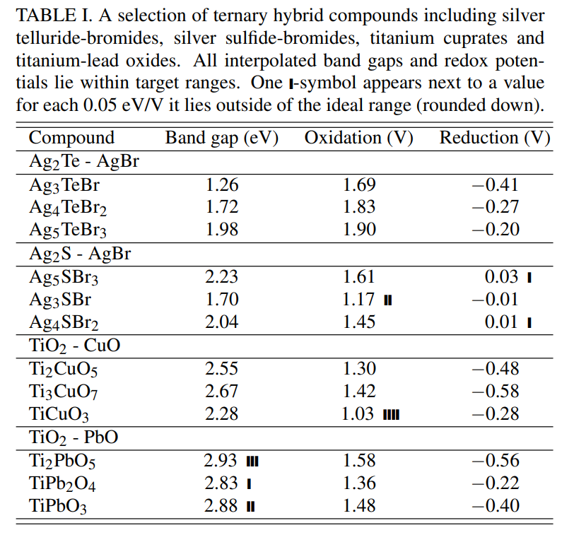
\ The four highest φox compounds in the high-Eg cluster were AgBr, TiO2, AgCl, and CuCl, ordered by the number of hybrids derived from them. 95% of hybrid compounds had a parent in this group, including 42% from AgBr alone. The four highest φox compounds with low-Eg were the binary combinations of Pb and Ag with Se and Te. 40% of hybrids had a parent in this group and 36% that had one parent from each group. Table I provides some example hybrid compounds from the target region including three hybrids of different composition from pairs of AgBr and TiO2 with lower Eg compounds. The variety of hybrids included represents how different parents produced hybrids in different regions, e.g. TiO2 – PbO hybrids tended to have low Eg.
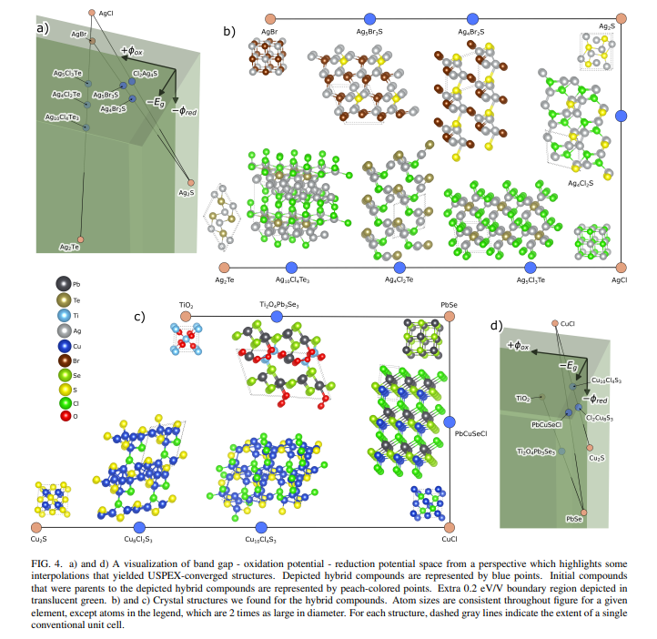
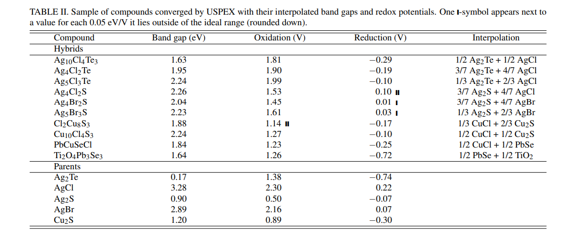
B. Candidate StructuresWe used the procedure for USPEX and VASP laid out in Section V E to search for the crystal structures of hybrids in our target region. USPEX was able to converge structures for about 50 hybrid compounds. The elemental composition of these structures mostly coincides with the composition in the hybrid compounds highlighted in the previous Section. For example, Ag has the greatest occurrence by far, due to its presence in both the low and high Eg groups. However, Br has a surprisingly much lower occurrence and Cd has a relatively higher occurrence. Figure 4 and Table II show example results of USPEX converged structures. Figure 4 also connects shifts in composition to changes in structure and property space.
\ USPEX allowed us to find hybrid structures that had different space groups from their parent structures. For example, PbCuSeCl has a space group of 156, which is different than any known PbSe or CuCl structure according to AFLOW.26 The approach of Hautier et al. 19 and most other materials searches using the substitution matrix technique would not have allowed the discovery of this structure because they enforced a restriction new candidate compounds had the same crystal structure as compounds from which they were derived.
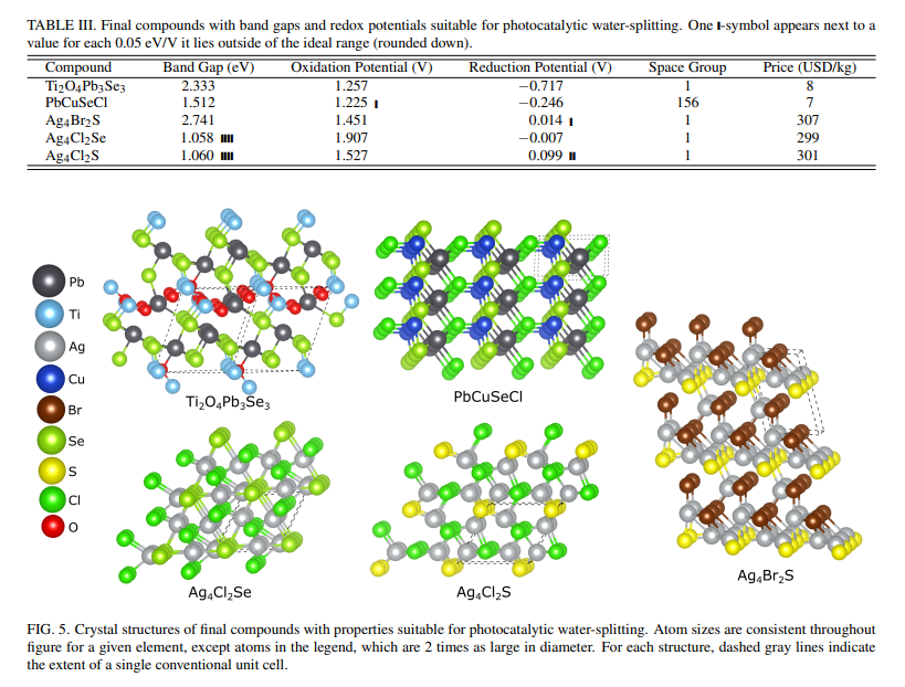
C. Final Water-SplittersFinally, we used the hybrid DFT code, CRYSTAL17, to conduct higher fidelity geometry optimization on our candidate structures. Many of the USPEX-converged structures had to be eliminated because the band gap derived from CRYSTAL17 moved them out of the target region of property space and others had to be eliminated because they would not converge. Structures containing Ag had larger discrepancies between their interpolated Eg and their CRYSTAL17-calculated Eg. On average the difference was 0.92 eV compared to 0.51 eV for non-Ag compounds. The largest difference was for Ag4Cl2Se which decreased by 1.17 eV, placing it slightly out of the ideal region. The surviving structures mostly had low symmetry. Figure 5 and Table III provide examples of final structures that remained in the target region of property space after CRYSTAL17 band gap calculation. We confirmed that no final structure existed in the AFLOW database.26
\
\
:::info This paper is available on arxiv under CC 4.0 license.
:::
\