BayesPPDSurv supports the incorporation of multiple historical datasets using the power prior with fixed a0 or using the normalized power prior with a0 modeled as random. It contains two categories of functions, functions for model fitting (”phm.fixed.a0” and ”phm.random.a0”) and functions for sample size determination (”power.phm.fixed.a0” and ”power.phm.random.a0”). Functions for model fitting return posterior samples of the parameters, while functions for sample size determination return estimates of the Bayesian power or type I error rate.

\ When a0 is modeled as random, the function approximate.prior.beta() performs slice sampling to generate samples of β from the normalized power prior. By default, the function phm.random.a0() approximates the normalized power prior for β, π(β|D0), with a single multivariate normal distribution. To accommodate greater accuracy of approximation, the package allows the user to approximate π(β|D0) with a finite mixture of multivariate normal distributions as well. Specifically, the user can take the output of the approximate.prior.beta() function, which is a matrix of samples of β from the normalized power prior, and use external software to compute a mixture of multivariate normal distributions that best approximates the samples. The resulting mixture distribution can then be the input to the prior.beta.mvn argument of phm.random.a0(), which is a list of lists, where each list has three elements, consisting of the mean vector, the covariance matrix and the weight of each multivariate normal distribution. Then, π(β|D0) is approximated by the mixture of the multivariate normal distributions provided. Since we use λ0 and a0 as auxiliary variables for the approximation for π(β|D0), the user specifies the hyperparameters for the priors for λ0 and a0 in the function approximate.prior.beta(). The hyperparameters for the priors for λ and the initial prior for β are specified in the function phm.random.a0().

\ The package allows the time interval partition to vary across the S levels of the stratification variable. The user must specify the total number of intervals for each stratum, n.intervals. Then for each stratum, by default, the change points are assigned so that an approximately equal number of events are observed in all the intervals for the pooled historical and current datasets. The user can also specify the change points for each stratum. When a0 is fixed, by default, the baseline hazard parameters are unshared (i.e., λ 6= λ0) between the current and historical data. If shared.blh=TRUE, baseline hazard parameters are shared and historical information is used to estimate the baseline hazard parameters. When a0 is modeled as random, the package only supports unshared baseline hazards.

\ For study design applications, the user can manipulate many attributes of the data generation process, including the enrollment time distribution (uniform or exponential), the randomization probability for the treated group, the censorship time distribution (uniform, exponential or constant), the probability of subjects dropping out of the study (non-administrative censoring), the dropout time distribution (uniform), and the minimum and maximum amount of time that subjects are followed.

3.1 Sampling Priors

Our implementation in BayesPPDSurv does not assume any particular distribution for the sampling priors. The user specifies discrete approximations of the sampling priors by providing a matrix or list of parameter values and the algorithm samples with replacement from the matrix or the list as the first step of the data generation. The user must specify samp.prior.beta, a matrix of samples for β, and samp.prior.lambda, a list of matrices where each matrix represents the sampling prior for the baseline hazards for each stratum. The number of columns of each matrix must be equal to the number of intervals for that stratum.

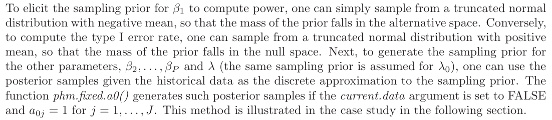
\ Now we describe strategies to elicit the sampling priors, as detailed in Psioda and Ibrahim (2019). Suppose one wants to test the hypotheses

\ H0 : β1 ≥ 0

\ and

\ H1 : β1 < 0.

\ \

:::info This paper is available on arxiv under CC by 4.0 Deed (Attribution 4.0 International) license.

:::

Feed: Hacker Noon - Medium

View: Original article

Tags: applications distribution framework