Inside the Math Banks Use to Decide If You’re a Credit Risk

Imagine you are managing a bank's credit portfolio: every loan issued is a bet on the borrower's ability to meet their obligations. But how can you determine which borrowers are reliable and which ones might struggle with repayments? This is where Probability of Default (PD) models come into play.

\ PD models are tools used in the banking sector to assess the likelihood of a borrower defaulting within a specific time frame. They play a critical role in risk management and the bank's credit policy.

\ In this article, I will explain how banks leverage PD models to evaluate credit risks, outline key approaches to building these models, and explore how machine learning is applied in their development.

What is "default" and why is it important to predict it?

Imagine a bank client (an individual) who has taken out a loan. Each month, they are required to pay a fixed amount by a specified due date. When payments are made on time, the loan is repaid, and the bank earns revenue in the form of interest. However, the process doesn’t always go smoothly: sometimes borrowers miss payments or pay less than the required amount. Such instances are referred to as delinquencies. If several months pass since the last partial payment, this is called entering the n-th delinquency stage, where n corresponds to the number of months in arrears.

\ Default is defined as a situation where the borrower is delinquent for 90 days or more (entering the 4th stage of delinquency). This is the point at which the borrower is officially recognized as unable to fulfill their loan repayment obligations to the bank.

\ For a bank, a client’s default is an extremely adverse event, leading to significant financial losses due to the non-repayment of the loan and additional costs associated with debt recovery. The ability to predict such events is one of the bank's key objectives.

\ To minimize these risks, banks use PD (Probability of Default) models. These tools analyze a wide range of data, including the client’s financial behavior, credit history, and current solvency, to forecast the probability of default and take timely preventive measures.

Behavioral-PD and Application-PD Models

In credit risk management, two main types of PD models are used: Application-PD models and Behavioral-PD models. Both types aim to assess the probability of a borrower defaulting but are applied at different stages and serve different purposes.

Application-PD Models

Application-PD models are used during the loan application review stage. Their primary objective is to assess the probability of a borrower's default even before the loan is issued, based on the information provided by the client in the application form, as well as data collected by the bank from external sources.

\ What data can be used?

• Client characteristics: age, marital status, education, etc.
• Employment details: income level, job tenure, and type of employment.
• Credit history: information on existing loans and repayment behavior.

\ These models rely on statistical methods and machine learning algorithms. By analyzing historical data, they identify correlations between borrower characteristics and their likelihood of default. The analysis produces a credit score, which the bank uses to decide whether to approve or deny the loan.

\ Application-PD models enable banks to:

• Quickly and objectively evaluate new clients.
• Reduce the risk of lending to unreliable borrowers.
• Standardize the decision-making process for loan applications.

Behavioral-PD Models

Behavioral-PD models are used to assess existing bank clients who already have loans. They analyze the borrower's behavior during the repayment process and help predict the likelihood of default in the future.

\ What data can be used?

• All data used in Application-PD models: client characteristics, employment details, and credit history.
• Behavioral data after the loan is issued: payment regularity and timeliness, outstanding debt, use of credit limits, transactional activity, and other parameters.

\ Behavioral models track changes in borrower behavior and detect signals that may indicate a potential deterioration in their financial situation. For example, reduced payment consistency or an increase in debt burden can serve as early indicators of future default.

\ Behavioral-PD models enable banks to:

• Respond promptly to changes in client behavior.
• Assess the overall risk level of the bank's credit portfolio.
• Identify reliable clients who can be further engaged in the bank’s ecosystem.

\ Behavioral-PD models can also be used in the bank's provisioning process, which I discussed in the article:

https://hackernoon.com/how-do-banks-predict-expected-credit-losses?embedable=true

Comparison of Application and Behavioral Models

| Aspect | Application Models | Behavioral Models | |----|----|----| | Stage of Application | Before loan issuance | During loan repayment | | Data | Demographic and financial | Current client behavior data | | Objective | Evaluating new borrowers | Monitoring existing borrowers | | Outcome | Loan approval decision | Prediction of risk level changes |

\ Thus, Application models help banks minimize risks at the loan application stage, while Behavioral models enable risk management throughout the entire loan term. The principles of building both application and behavioral models are largely similar. In this article, the focus will be on Behavioral-PD models.

Building a Behavioral-PD Model

A Behavioral-PD model is designed to predict the probability of default for each issued loan. Simply put, its task is to assess, on a daily basis, from the moment the loan is issued until it is fully repaid, the likelihood that the borrower will fail to meet their obligations within a specific time frame.

What does "within a specific time frame" mean?

This means that the model forecasts the probability of default not for an indefinite future but within a defined time horizon. For instance, this horizon is often set at 12 months from the moment the prediction is made.

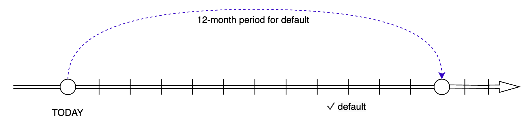
Setting a standardized default prediction window ensures consistency in the metric being forecasted. A 12-month horizon is the most commonly used, but it is not the only option. For example, for loans showing signs of credit quality deterioration, forecasts can be built for the entire loan lifecycle until its closure. However, this aspect will not be explored in detail in this article.

Problem Formulation

Thus, the model's task is to classify all loans into two categories:

• "1" — the loan defaults within 12 months.
• "0" — the loan does not default within 12 months.

This transforms the problem into a binary classification task, where the model predicts the probability of each loan belonging to class "1" (i.e., default).

Methods and Approaches

Binary classification is a classic machine learning problem with numerous approaches available. However, the choice of algorithm is often influenced by regulatory and audit requirements, which demand high model interpretability.

\ Despite the high accuracy of complex methods such as gradient boosting and neural networks, banks frequently rely on linear classifiers like logistic regression due to their transparency and interpretability. Nevertheless, interest in more sophisticated models is growing, and the industry is gradually shifting towards their adoption.

Model Training

Let’s move on to building the model. What do we expect from the predicted probabilities?

1. Sorting Quality: The predicted probabilities should correctly rank clients by default risk. Borrowers more likely to default should have a higher PD compared to those who are more likely to meet their obligations.
2. Probability Calibration: The predicted probabilities should match the actual default rates. For example, if a group of clients has a predicted default probability of 20%, the actual default rate for this group should also be around 20%.

\ Achieving both high-quality ranking and accurate calibration within a single model is challenging. The main issue lies in the fact that default rates within the same customer segment can change significantly over short periods due to external factors, such as economic conditions or changes in the bank’s policies.

\ To address this, a family of models can be built, with each model solving a specific subtask.

\ For example, a complex "stationary" model can first be built using a large set of historical data and a wide range of features. This model can include various client and loan characteristics to rank borrowers effectively by default risk over a 12-month horizon. The goal of this model is to ensure stable and accurate ranking.

\ Next, a simple "calibration" model can be trained to adjust the probabilities predicted by the "stationary" model based on the most up-to-date data. For example, calibration can incorporate recent information on defaults over the last 12 months. This involves using the latest data, where actual default cases for the specified period are already known. The "calibration" model is trained using the predictions of the "stationary" model as the sole feature. Utilizing such a model helps improve the probability calibration of the behavioral model.

\ The "stationary" model can be trained once and used as long as it ensures quality ranking. At the same time, the "calibration" model can be updated regularly to keep the predicted probabilities accurate and unbiased relative to the current risk levels.

\ The idea of applying calibrations can be extended. For instance, if your task requires predicting the probability of default not over 12 months but over 24 months or the entire lifetime of the loan, you can use the same principle as when creating a calibration model. The only difference is selecting a target that aligns with your specific task.

\ A separate task is monitoring the quality of such models. I described how this can be done in the article:

https://hackernoon.com/probabilistic-predictions-in-classification-evaluating-quality?embedable=true

Additional Aspects

Portfolio Segmentation

When building PD models, it is advisable to segment the portfolio, creating separate models for each segment. This is necessary because different types of loans and borrowers exhibit different behaviors. Here are classic examples of such segmentation:

• Product type: Consumer loans, credit cards, and mortgages are fundamentally different products with varying terms, amounts, and repayment structures. Each type requires its own model that considers its unique characteristics.
• Presence of delinquencies: Payment delinquencies significantly increase risk (PD), and the behavior of borrowers with delinquencies often differs from those who pay on time.

\ Experience shows that developing separate models for major segments leads to more accurate results and better accounts for variations in client behavior.

\ Lagging Behind Reality

PD models rely on historical data, which takes time to "mature" for the target variable (e.g., 12 months in our case). This results in a lag between the probability calibration and the current risk levels. To minimize this lag, approaches are used that focus on events strongly correlated with the target variable but less delayed relative to the current date. These methods allow probability forecasts to be updated based on fresher data.

Conclusion

This article has covered the basic aspects of creating and applying PD models for credit risk forecasting. We explored how Application-PD models help evaluate new borrowers at the application stage, while Behavioral-PD models monitor the behavior of active clients and detect early risk indicators. Additionally, we reviewed an example of building a Behavioral-PD model.

\ Of course, in real-life scenarios, the process is more complex, and many details have been intentionally simplified here.