and the distribution of digital products.
DM Television
How to Make Big Data Clustering Faster and More Efficient
:::info Authors:
(1) Andrew Draganov, Aarhus University and All authors contributed equally to this research;
(2) David Saulpic, Université Paris Cité & CNRS;
(3) Chris Schwiegelshohn, Aarhus University.
:::
Table of Links2 Preliminaries and Related Work
2.3 Coresets for Database Applications
4 Reducing the Impact of the Spread
4.1 Computing a crude upper-bound
4.2 From Approximate Solution to Reduced Spread
5 Fast Compression in Practice
5.1 Goal and Scope of the Empirical Analysis
5.3 Evaluating Sampling Strategies
5.4 Streaming Setting and 5.5 Takeaways
8 Proofs, Pseudo-Code, and Extensions and 8.1 Proof of Corollary 3.2
8.2 Reduction of k-means to k-median
8.3 Estimation of the Optimal Cost in a Tree
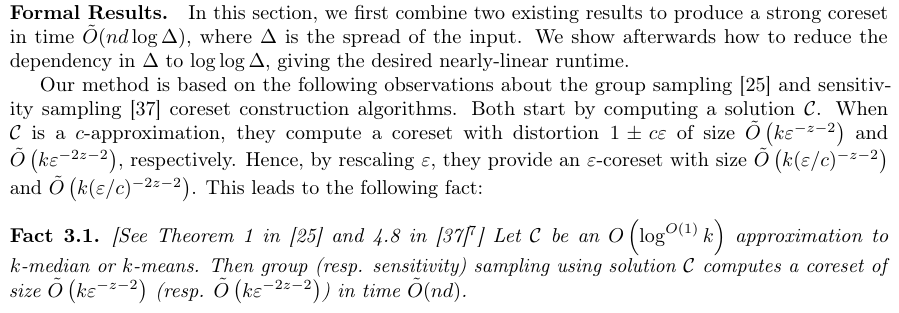
3 Fast-CoresetsTechnical Preview. We start by giving an overview of the arguments in this section.
\ There exists a strong relationship between computing coresets and approximate solutions – one can quickly find a coreset given a reasonable solution and vice-versa. Thus, the general blueprint is as follows: we very quickly find a rough solution which, in turn, facilitates finding a coreset that approximates all solutions. Importantly, the coreset size depends linearly on the quality of the rough solution. Put simply, the coreset can compensate for a bad initial solution by oversampling. Our primary focus is therefore on finding a sufficiently good coarse solution quickly since, once this has been done, sampling the coreset requires linear-time in n. Our theoretical contribution shows how one can find this solution on Euclidean data using dimension reduction and quadtree embeddings.
\

\

\ To turn Fact 3.1 into an algorithm, we use the quadtree-based Fast-kmeans++ approximation algorithm from [23], which has two key properties:
\

\ The second property is crucial for us: the algorithm does not only compute centers, but also assignments in O˜(nd log ∆) time. Thus, it satisfies the requirements of Fact 3.1 as a sufficiently good initial solution. We describe how to combine Fast-kmeans++ with sensitivity sampling in Algorithm 1 and prove in Section 8.1 that this computes an ε-coreset in time O˜(nd log∆):
\ Corollary 3.2. Algorithm 1 runs in time Oe (nd log ∆) and computes an ε-coreset for k-means
\ Furthermore, we generalize Algorithm 1 to other fast k-median approaches in Section 8.4.
\ Thus, one can combine existing results to obtain an ε-coreset without an Oe(nk) time-dependency. However, this has only replaced the Oe(nd + nk) runtime by Oe(nd log ∆). Indeed, the spirit of the issue remains – this is not near-linear in the input size.
\

\

\
:::info This paper is available on arxiv under CC BY 4.0 DEED license.
:::

- Home
- About Us
- Write For Us / Submit Content
- Advertising And Affiliates
- Feeds And Syndication
- Contact Us
- Login
- Privacy
All Rights Reserved. Copyright , Central Coast Communications, Inc.