and the distribution of digital products.
DM Television
How to Implement Propensity Score Matching: A Step-by-Step Guide
\
Recently I was working on an experiment based on Propensity Score Matching and while researching information I encountered a lack of materials on the topic. Most of the articles I found are on effectiveness of the method and they’re not well-detailed in terms of theory. Therefore, I decided to share with you a comprehensive guideline on Propensity Score Matching framework and its steps What is Propensity Score Matching and why apply it?“Propensity score matching entails forming matched sets of treated and untreated subjects who share a similar value of the propensity score. Once a matched sample has been formed, the treatment effect can be estimated by directly comparing outcomes.”
\ The definition was first given by Rosenbaum P.R., Rubin D.B. in article “Assessing sensitivity to an unobserved binary covariate in an observational study with binary outcome” of 1983.
\ To put it simply, this is an additional A/B tests technique employed when sample randomisation doesn’t work. Propensity score (probability of being assigned to test group) of a treatment group is counted for every user and then the user is matched with another user based on historical data of product usage forming a control group. Afterwards, the results of two groups are compared using a statistical test and an experiment effect is measured.
\

\ But why use the complex technique of finding a control group if an A/B platform can do it instead? In some cases it’s not possible to employ an A/B platform with a built-in splitting function. Here are the possible cases:
\
- It’s expensive and time-consuming for business to implement an A/B test due to various cross functional work and communications (yes, it may happen).
- A company may lack profit while testing monetisation or marketing-related functions/strategies in case of implementing classic test/control experiment.
- It’s often impossible to have a randomised sampling in offline experiments which is required for an A/B test.
- It’s also not workable to apply an A/B test in online experiments when a tested object is not randomly distributed.
\ I had the fourth case in my practice and it happened while working with an e-commerce product. A product team was preparing to test a function of giving bonuses to users after placing the first order. The problem was that the function was working not on all users placing the first order. Certain conditions, such as the value of the order, etc., had to be met. In this case, it’s beyond the limits of an A/B test platform to split the traffic between the test and the control groups. Here’s why Propensity Score Matching was the option.
Framework of the Propensity Score MatchingA complete framework is roughly based on an article “Propensity score matching with R: conventional methods and new features” and comprises five steps (Figure 2).
\ The first step is to collect the data on which a propensity score is estimated and a matched user is found.
\ The second step is to estimate a propensity score using methods, such as logistic regression, and train on the dataset to predict whether a user will be assigned to a test group. For every user, the trained model generates a probability of being in a test group.
\ The third step refers to matching based on propensity score, where different matching methods are tried, such as nearest neighbor.
\ In the fourth step, the balance of covariates between treatment and control groups is checked by calculating balance statistics and generating plots. A poor balance indicates that the model estimating propensity score needs to be respecified.
\ In the fifth final step, the effects of a test are estimated using matched data and a statistical test is conducted.
\

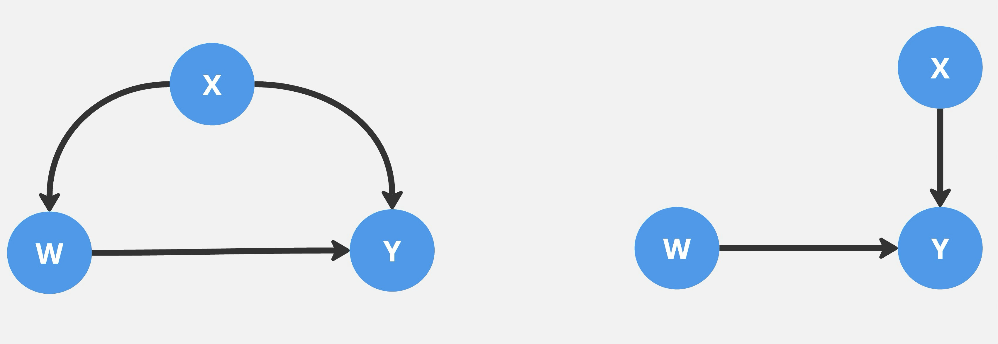
This stage is regarding collecting required variables, covariates and confounders. Covariate (X) is an independent variable that can influence the outcome of an experiment (Y), but which is not of direct interest. Confounder is a factor other than the one being studied that is associated both with the allocation to a test group (W) and with the outcome of an experiment (Y).
\ The graph below illustrates the relationships of variables. X is a covariate, W is an indicator of treatment assignment, and Y is the outcome. The graph on the left depicts confounder’s relationship and the one on the right shows independent connection of covariate to the experiment’s result (Y) and to test group allocation (W).
\

\
:::tip Here it’s crucial to underline that it’s not recommended to select only variables that are associated with assignment of the users to a test group (W) because it may reduce the precision in evaluation of group difference without decreasing bias (https://www.ncbi.nlm.nih.gov/pmc/articles/PMC1513192/ ).
:::
\ You may ask how many variables do I need to select? The answer is simple - the more, the better in order to obtain high estimation of the results and minimise study bias. And here I’m talking about big numbers as 20-50 or even more.
Propensity Score EstimationMoving on to the next step, it’s required to gather the data and set a flag of belonging to a treatment group. All other users will potentially form a control group. Afterwards propensity score is estimated using various methods, such as logistic regression or random forests.
\ Most of the articles I’ve read suggest sticking to logistic regression and not using other more complex models as high accuracy is not crucial. Yet, succeeding matching technique concentrates on accuracy.
\ After selecting the method, a predictive model is trained on the data using the selected covariates to predict whether a user belongs to a test group. Lastly, the model makes predictions for each user, and propensity score, the probability of being in a test group, is calculated. In terms of softwares, in Python you can use any forecasting library starting from basic scikit-learn and moving to Prophet.
Data MatchingThe following action is to implement a matching technique to find a matched user to user from a test group. Therefore, a control group is formed.
\ There are various matching methods to choose from, for instance exact matching or Mahalanobis distance matching. In this article I’m mainly going to discuss common technique of nearest neighbour matching and its variations.
\ Nearest neighbor matching (NNM) is composed of two phases. First, the algorithm picks users, one by one from a treatment group, in a specified order. Subsequently, for each user of a test group, the algorithm finds a user in the control group with the nearest propensity score. These steps are repeated until no users are left in the test or control groups. In Python, there are specific libraries for PSM as PyTorch, Psmpy, causallib. Or you always can stick to any classic library with matching algorithms.
\
:::tip It’s pivotal to underline that in case of creating a control group similar to a classic A/B test, where users in a group are unique and sample sizes are equal, NNM without replacement method must be implemented. The method implies that after matching, the matched pair will be removed, so that a user in the control group will be used only once.
:::
\ There’s also an option to select an NNM model with or without caliper. A caliper sets the upper limit of the distance of propensity scores in a matched pair. Thus, every user can only be matched to users of a propensity score within a limited range. If eligible users can’t be matched, the user will be discarded.
\ Why should I employ the caliper? It’s advisable to apply it when the distance of propensity scores in a matched pair may be large. When deciding on a caliper size, consider the following: if the matching performance is not satisfactory, matching can be conducted with a tighter caliper and if matching is successful but the number of matched pairs is small, the caliper can be broadened (https://www.ncbi.nlm.nih.gov/pmc/articles/PMC8246231/ ).
Balance DiagnosticsDuring this stage it’s checked whether covariates of test and matched control groups are balanced, thus, it claims whether a match is accurate.
:::info It’s a crucial step as unbalanced covariates will lead to incorrect A/B test results comparison.
:::
There are three means of balance diagnostics:
\ - descriptive statistics: standardised mean difference (SMD) or variance ratio (VR)
- statistical tests
- visualisation: qq-plot, histogram or love plot
\ In the article I mainly concentrate on the first and the third options.
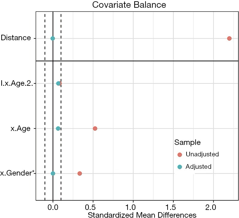
\ First, let’s discuss standardised mean difference and variance ratio. What values indicate that a covariate is balanced? I recommend that SMD value is below 0.1 In terms of VR, a values close to 1.0 indicates a balance.
\ In the second place, regarding visualisation methods, one of the above descriptive statistics is calculated for every covariate and displayed graphically. I personally prefer a love plot as all covariates can be placed in one graph and covariates before and after matching can be easily compared. I place an example of the graph below.
\

\ What if covariates are still unbalanced after matching? To illustrate, standardised mean difference (SMD) of covariates frequency of purchases and AOV are around 0.5, which is above required 0.1. It implies that the covariates are imbalanced and rematching is needed.
:::warning Imbalanced covariates signal PSM model is not effective and needs to be rebuilt. Therefore, it’s a must to go a few steps back and repeat matching.
:::
There are four methods to redo matching:
\ 1. Add new covariates
2. Simply change the matching method as there are plenty of them
3. Combine Propensity Score Matching with exact matching method
4. Increase a sample size
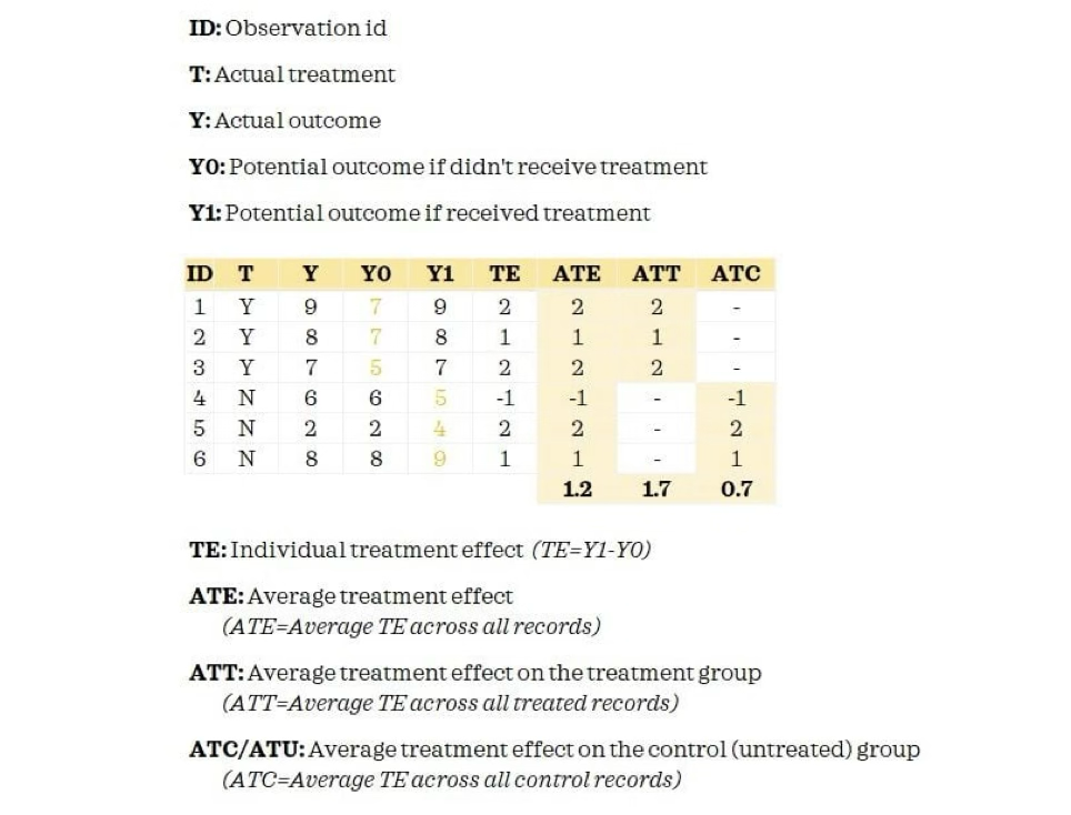
Estimate of Treatment EffectsFinally, we are approaching the last stage when experiment effect is estimated. There are mainly three types of effect estimation: the average treatment effect (ATE), the average treatment effect on the treated (ATT), and the average treatment effect on the control (ATC). Basically speaking, ATE is a computed difference in a key metric between test and control groups (similar measuring a main metric in an A/B test). It’s calculated as a mean of treatment effect, ATE = avg (Y1 - Y1) as illustrated below in the figure.
\

\ While ATT and ATC are an average treatment effect of a test and control group, respectively. All are straightforward and understandable estimation methods.
\ ATE is the most common type and used when control and test groups’s major metric is compared and tested effect is measured. While ATT and ATC are preferred when absolute metrics are required for every group. Ultimately, an appropriate statistical test is conducted to check statistical significance of the results.
Limitations of Propensity Score MatchingAfter the detailed explanation of the Propensity Score Matching method, it may be time to start implementing it in your work, but there are certain limitations must be considered.
\ 1. Bootstrap is not recommended to be employed with Propensity Score Matching as it increases variance. (https://economics.mit.edu/sites/default/files/publications/ON THE FAILURE OF THE BOOTSTRAP FOR.pdf)
2. Stable unit treatment value assumption (SUTVA) principle must be met. 3. Propensity Score Matching implies using two machine learning algorithms (one for propensity score calculations and the second one for matching), which can be a pricy method to use for a company. On that account, it’s advisable to negotiate with your team on A/B test conduction. 4. Finally, as discussed above, a big number of covariates are suggested to be used in the models. Thus, it requires a high-powered machine(-s) to calculate the results of the models. Again, it’s a costly method to implement. However, if it’s possible to implement Propensity Score Matching, do it and don’t hesitate to enhance your experience and practical knowledge. Good luck with your future experiments and machine learning discoveries\
:::info Would you like to take a stab at answering some of these questions? The link for the template is HERE. Interested in reading the content from all of our writing prompts? Click HERE.
:::
\n
\ \n
- Home
- About Us
- Write For Us / Submit Content
- Advertising And Affiliates
- Feeds And Syndication
- Contact Us
- Login
- Privacy
All Rights Reserved. Copyright , Central Coast Communications, Inc.