and the distribution of digital products.
How Central Banks Shape the Economy
:::info Author:
(1) David Staines.
:::
Table of Links4 Calvo Framework and 4.1 Household’s Problem
4.3 Household Equilibrium Conditions
4.5 Nominal Equilibrium Conditions
4.6 Real Equilibrium Conditions and 4.7 Shocks
5.2 Persistence and Policy Puzzles
6 Stochastic Equilibrium and 6.1 Ergodic Theory and Random Dynamical Systems
7 General Linearized Phillips Curve
8 Existence Results and 8.1 Main Results
9.2 Algebraic Aspects (I) Singularities and Covers
9.3 Algebraic Aspects (II) Homology
9.4 Algebraic Aspects (III) Schemes
9.5 Wider Economic Interpretations
10 Econometric and Theoretical Implications and 10.1 Identification and Trade-offs
10.4 Microeconomic Interpretation
\ Appendices
A Proof of Theorem 2 and A.1 Proof of Part (i)
B Proofs from Section 4 and B.1 Individual Product Demand (4.2)
B.2 Flexible Price Equilibrium and ZINSS (4.4)
B.4 Cost Minimization (4.6) and (10.4)
C Proofs from Section 5, and C.1 Puzzles, Policy and Persistence
D Stochastic Equilibrium and D.1 Non-Stochastic Equilibrium
D.2 Profits and Long-Run Growth
E Slopes and Eigenvalues and E.1 Slope Coefficients
E.4 Rouche’s Theorem Conditions
F Abstract Algebra and F.1 Homology Groups
F.4 Marginal Costs and Inflation
G Further Keynesian Models and G.1 Taylor Pricing
G.3 Unconventional Policy Settings
H Empirical Robustness and H.1 Parameter Selection
I Additional Evidence and I.1 Other Structural Parameters
I.3 Trend Inflation Volatility
A.2 Behaviour of ∆The following theorem accomplishes the proof of Theorem 2(ii) and Proposition 15.
\
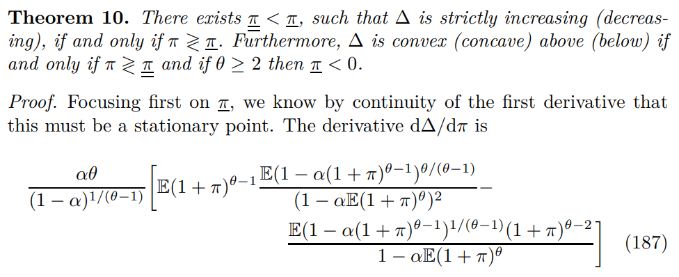
\ To prove existence of the bounds examine the limiting behavior of the derivatives around the poles. At the positive pole
\
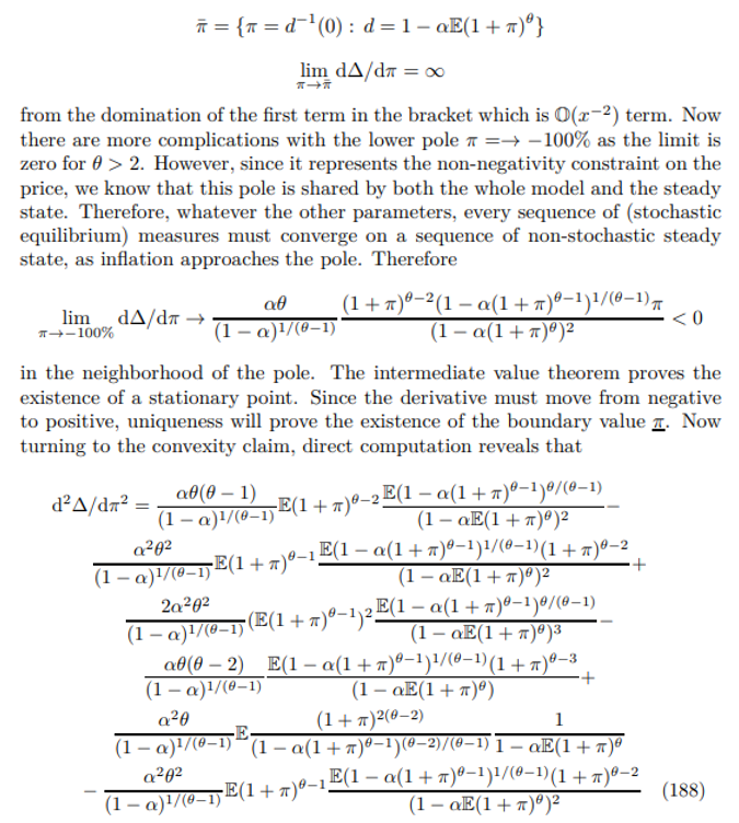
\
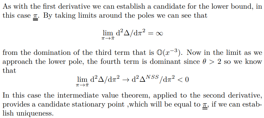
\
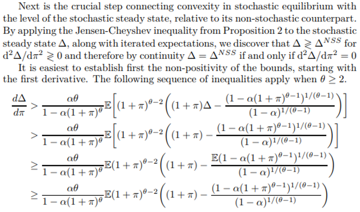
\
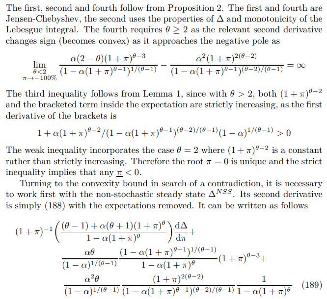
\ where the first term comes from the first and fourth terms of the previous expression, the second comes from combining terms two, three and six whilst the final term is term five. By taking the non-stochastic limit of the first derivative (187)
\

\ it is clear that sgn(d∆/dπ) = sgn(π). As the first derivative is (strictly) positive for (strictly) positive inflation, we know that is strictly convex for non-negative inflation.
\
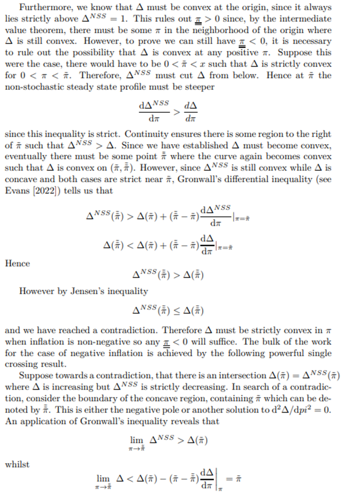
\ Hence
\

\ Finally, turning to the sharpness of the parameter condition required by Theorem 2, consider the limit case where
\
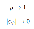
\ suppose further that
\

\ so the distribution of A approaches a two point discrete distribution. The persistent limit means we can transfer this to the distribution of inflation
\

\ Furthermore let the upper bound of the shock be arbitrarily increased
\

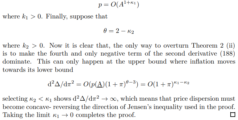
\ so by taking the non-stochastic limit of the steady state (detailed in Appendix D) it is clear that
\

\ whilst the probability is scaled down to preserve the boundedness of the expectation by
\
\
:::info This paper is available on arxiv under CC 4.0 license.
:::
\
- Home
- About Us
- Write For Us / Submit Content
- Advertising And Affiliates
- Feeds And Syndication
- Contact Us
- Login
- Privacy
All Rights Reserved. Copyright , Central Coast Communications, Inc.