and the distribution of digital products.
Fictitious Play for Mixed Strategy Equilibria in Mean Field Games: Mixed Strategy Equilibrium
:::info Authors:
(1) Chengfeng Shen, School of Mathematical Sciences, Peking University, Beijing;
(2) Yifan Luo, School of Mathematical Sciences, Peking University, Beijing;
(3) Zhennan Zhou, Beijing International Center for Mathematical Research, Peking University.
:::
Table of Links2 Model and 2.1 Optimal Stopping and Obstacle Problem
2.2 Mean Field Games with Optimal Stopping
2.3 Pure Strategy Equilibrium for OSMFG
2.4 Mixed Strategy Equilibrium for OSMFG
3 Algorithm Construction and 3.1 Fictitious Play
3.2 Convergence of Fictitious Play to Mixed Strategy Equilibrium
3.3 Algorithm Based on Fictitious Play
4 Numerical Experiments and 4.1 A Non-local OSMFG Example
5 Conclusion, Acknowledgement, and References
2.4 Mixed Strategy Equilibrium for OSMFGIf we relax the constraint forcing agents to uniformly exit at {u = ψ}, mixed strategy equilibrium can be defined. With multiple optimal choices available, mixed equilibria allow agents to randomize over strategies freely, rather than requiring identical decisions.
\ Assume that the cost functions f and ψ depend only on the crowd distribution m, the PDE system governing the mixed strategy equilibrium for OSMFG is as follows:
\
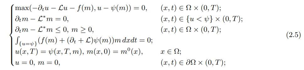
\ We refer to [5] for more discussions of the mixed strategy equilibrium. The last equation of (2.5) shows that
\
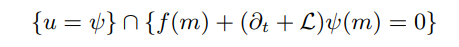
\ is the region where agents can choose to exit or to stay. It can be derived by standard stochastic calculus that agents would have the same cost whenever exiting or staying at (x, t) when (x, t) ∈ {f(m)+ (∂t+L)ψ(m) = 0}. This is the main relaxation compared to pure strategy equilibrium. The following existence result shows that such relaxation is sufficient, and hence mixed strategy equilibrium is a better notion for mean field games with optimal stopping time. In order to state the theorem rigorously, we first introduce two spaces and some technical assumptions for f and ψ.
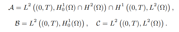
\ Definition 2.1 We define function spaces A, B and C as:
\
\ Assumption 2.1 The running cost f(·, ·, m) and the stopping cost ψ(·, ·, m) satisfy:
\
The map m → f(·, ·, m) is continuous from C to itself;
\
The map m → ψ(·, ·, m) is continuous from C to A
\ A. Then the existence result can be formulated in the following theorem.
\ Theorem 2.2 Suppose that Assumption 2.1 holds. Then there exists at least one solution (u, m) ∈ A × B for (2.5)
\ We refer the readers to Theorem 2.1 of [5] for the proof of the theorem above. Although the existence of the mixed strategy equilibrium can be guaranteed, it is yet difficult to design a simple and efficient numerical PDE algorithm for (2.5) directly due to its complicated form. The coupling between u and m is more intricate due to the complementary condition
\
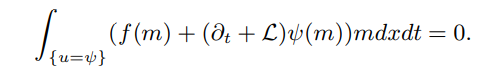
\ In the next section, the primary goal is to construct an iterative algorithm that provides an accurate approximation of the mixed strategy equilibria for OSMFGs via a generalized fictitious play.
\
:::info This paper is available on arxiv under CC 4.0 license.
:::
\