Electric Truths: What 16 Power Grid Models Reveal About DPFL

:::info Authors:

(1) Mengshuo Jia, Department of Information Technology and Electrical Engineering, ETH Zürich, Physikstrasse 3, 8092, Zürich, Switzerland;

(2) Gabriela Hug, Department of Information Technology and Electrical Engineering, ETH Zürich, Physikstrasse 3, 8092, Zürich, Switzerland;

(3) Ning Zhang, Department of Electrical Engineering, Tsinghua University, Shuangqing Rd 30, 100084, Beijing, China;

(4) Zhaojian Wang, Department of Automation, Shanghai Jiao Tong University, Dongchuan Rd 800, 200240, Shanghai, China;

(5) Yi Wang, Department of Electrical and Electronic Engineering, The University of Hong Kong, Pok Fu Lam, Hong Kong, China;

(6) Chongqing Kang, Department of Electrical Engineering, Tsinghua University, Shuangqing Rd 30, 100084, Beijing, China.

:::

Abstract and 1. Introduction

2. Evaluated Methods

3. Review of Existing Experiments

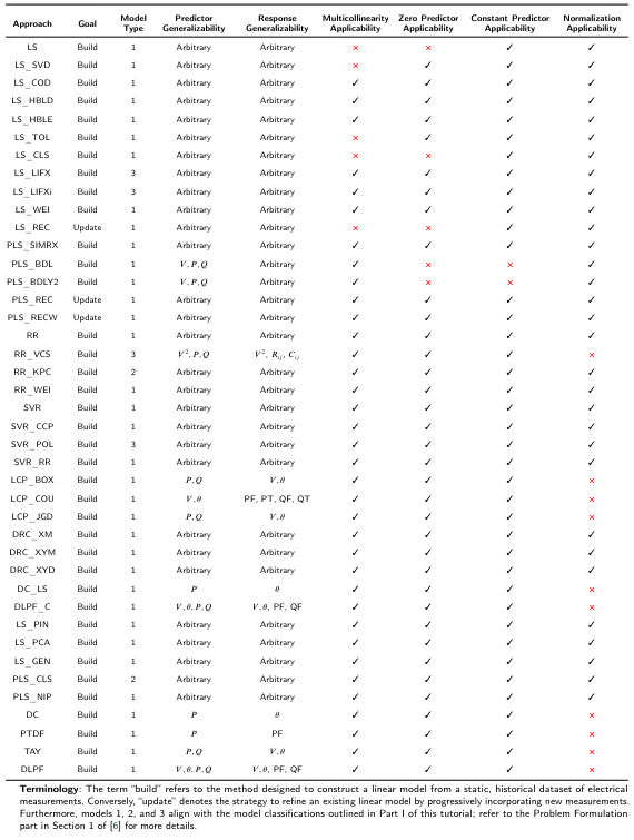
4. Generalizability and Applicability Evaluations and 4.1. Predictor and Response Generalizability

4.2. Applicability to Cases with Multicollinearity and 4.3. Zero Predictor Applicability

4.4. Constant Predictor Applicability and 4.5. Normalization Applicability

5. Numerical Evaluations and 5.1. Experiment Settings

5.2. Evaluation Overview

5.3. Failure Evaluation

5.4. Accuracy Evaluation

5.5. Efficiency Evaluation

6. Open Questions

7. Conclusion

Appendix A and References

For the numerical analysis, we chose a diverse range of transmission and distribution system models, spanning from 9-bus systems to 1354-bus systems, with 16 distinct configurations. In the following, we first detail the settings for each test case and the methods evaluated. Subsequently, we present the evaluation results with discussions from various perspectives. The open-source code for all the simulations in this paper can be found here [53].

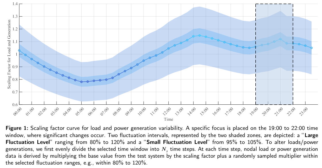
The detailed settings of all test cases are summarized in Table 4. To create the time-series variability in nodal loads and power generations in each test case, a typical daily load curve (in p.u.), shown in Fig. 1, is used as a time-varying scaling factor to change both nodal demand and supply. We also introduce some randomness by adding different fluctuation levels to the scaling factor[2]. Detailed descriptions are provided in the caption of Fig. 1. The resulting supply and demand data are then inputted into AC power flow solvers to generate measurements like nodal voltage, angle, active and reactive power injections, and branch flows. All these measurements are further divided into training and testing datasets. The training dataset is used for DPFL methods to estimate the linear model, while the testing dataset is used to evaluate the linearization errors of DPFL and PPFL methods. The reader is referred to Table 5 for a thorough illustration of the settings for each method, including their predictors, responses, hyperparameters (or the cross-validation ranges[3]), datasets, solvers (when applicable), and additional relevant information.

\

\

\

:::info This paper is available on arxiv under CC BY-NC-ND 4.0 Deed (Attribution-Noncommercial-Noderivs 4.0 International) license.

:::

[2] Note that for a specific system we use the same scaling curve for all of the methods but across the different systems the randomness is different.

\ [3] In this study, cross-validation is employed for hyperparameter tuning only in cases where the literature does not specify the hyperparameter values.