and the distribution of digital products.
Eigenvector Perturbation in Aligning Matrix Construction for ESPRIT
1.1 ESPRIT algorithm and central limit error scaling
1.4 Technical overview and 1.5 Organization
2 Proof of the central limit error scaling
3 Proof of the optimal error scaling
4 Second-order eigenvector perturbation theory
5 Strong eigenvector comparison
5.1 Construction of the “good” P
5.2 Taylor expansion with respect to the error terms
5.3 Error cancellation in the Taylor expansion
C Deferred proofs for Section 2
D Deferred proofs for Section 4
E Deferred proofs for Section 5
F Lower bound for spectral estimation
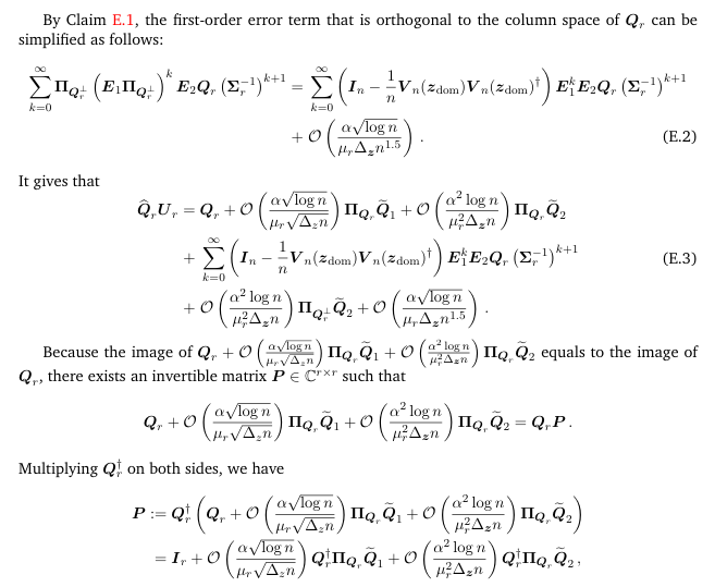
E Deferred proofs for Section 5 E.1 Proof for Step 1: Construction of the “good” P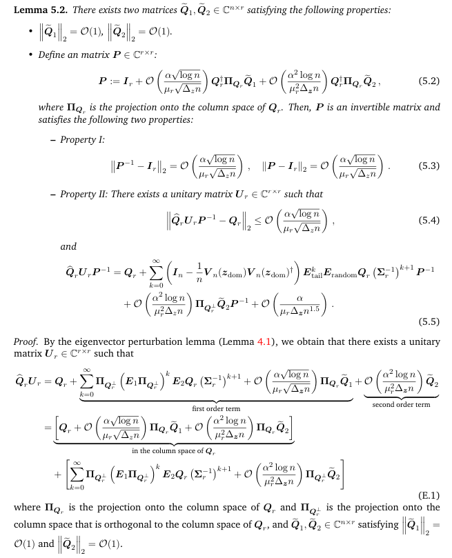
\
\ which gives the expression of P Eq. (5.2) in the lemma.
\ Property I and II follow from Claim E.2. The proof of the lemma is then complete
\ E.1.1 Technical claims
\

\ Proof. Note that
\

\ For the first term, we have
\
\
\ For the second term, we have
\
\ Combining them together, we have
\
\ The claim is then proceed.
\ Claim E.2 (Properties of the “good” P). The invertible matrix P defined by Eq. (5.2) satisfies the following properties:
\
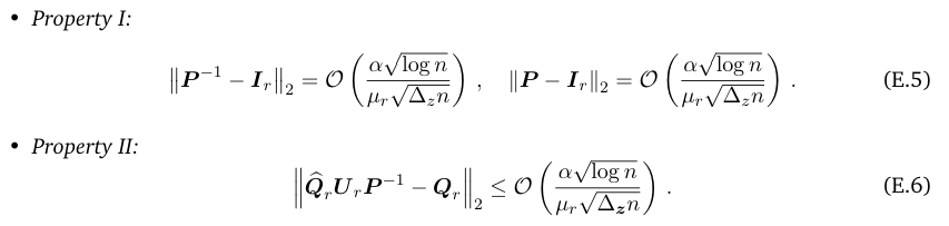
\ Proof. We prove each of the properties below.
\ Proof of Property I:
\ By the definition of P (Eq. (5.2)), we have
\
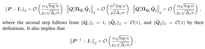
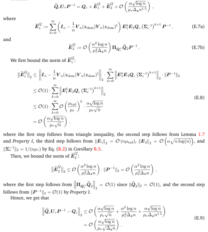
\ Proof of Property II:
\ Consider
\
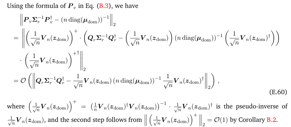
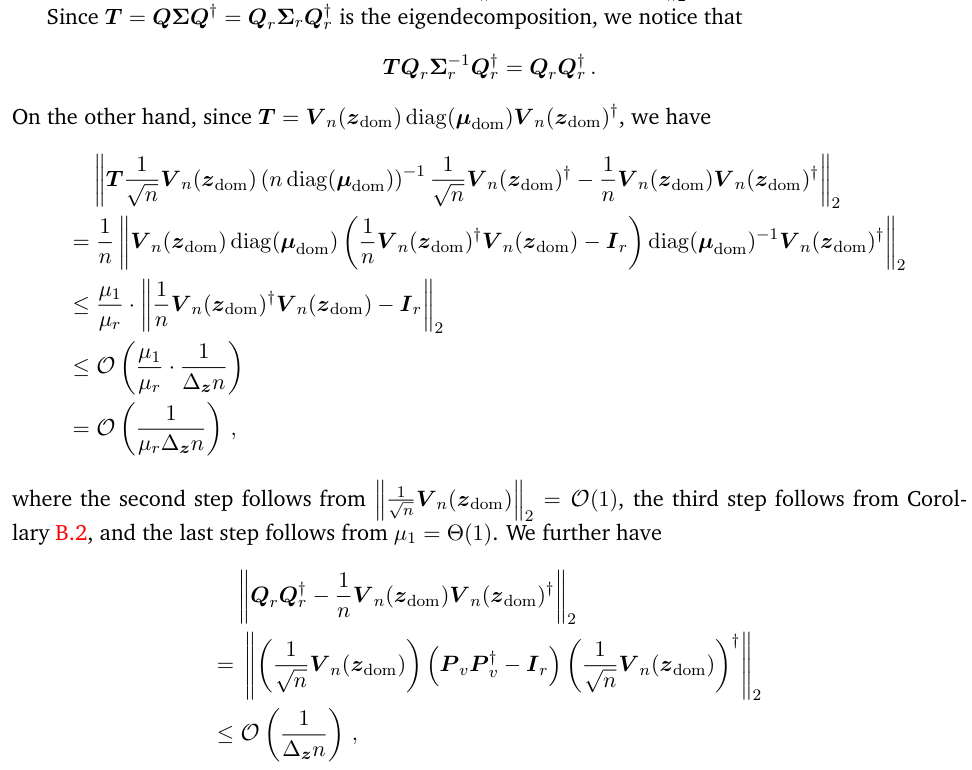
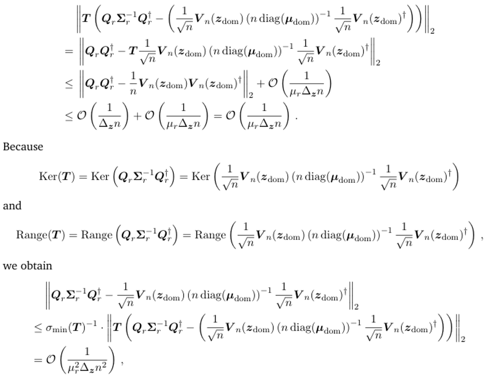
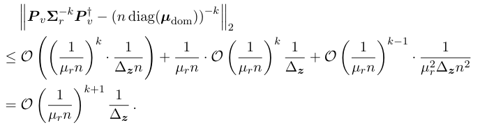
Lemma 5.3. Let P be defined as Eq. (5.2). Then, we have
\
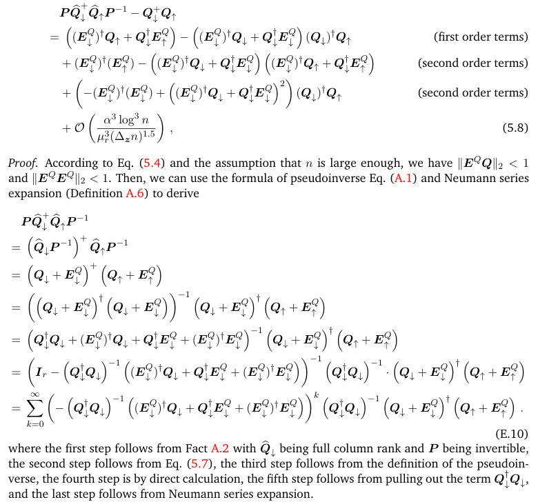
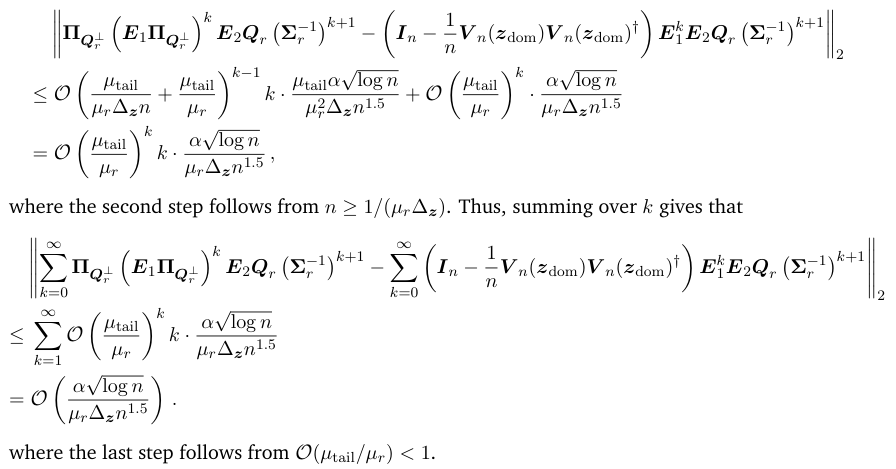
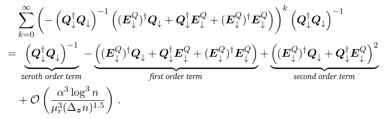
\ By Claim E.4, the Neumann series in Eq. (E.10) can be truncated up to second order:
\
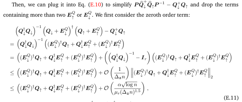
\
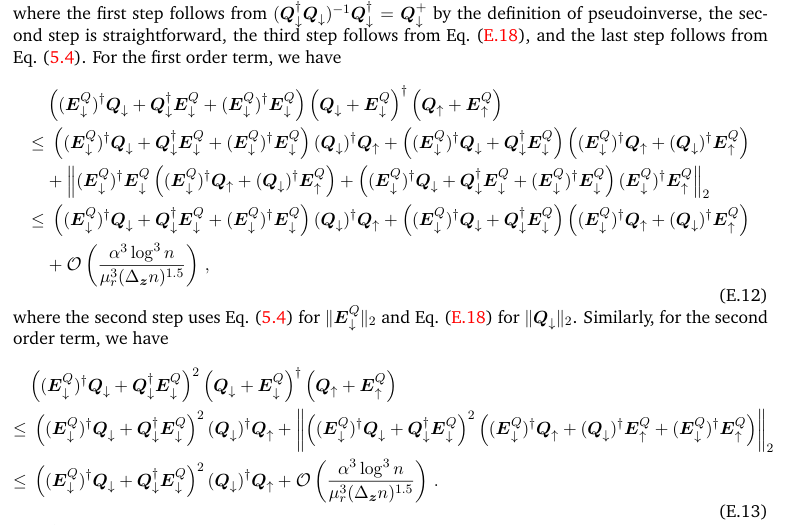
\ And for the residual term, we have
\

\ Finally, combining Eqs. (E.11) to (E.14) together, we obtain that
\
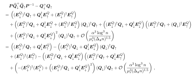
\ where we re-group the terms in the second step.
\ The proof of the lemma is completed.
\ Lemma 5.4. It holds that
\

\ Proof. We first deal with the first order term in Eq. (5.8):
\
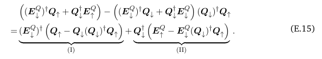
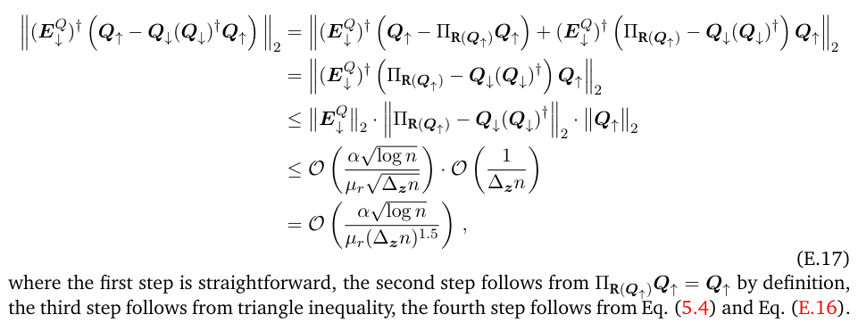
\ To bound (I), we notice
\
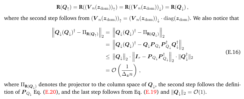
\ Combining this and Eq. (5.4), we obtain
\
\ Next, we keep (II) and first consider the second-order term in Eq. (5.8), which can be rewritten as follows:
\
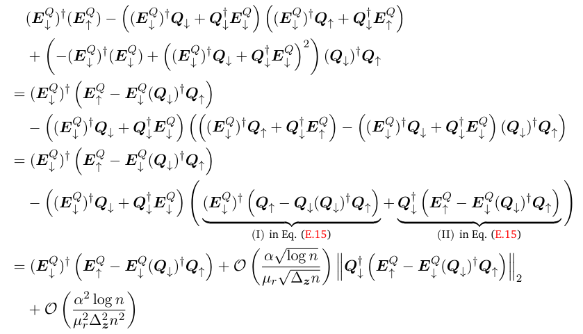
\ where the first two steps follow from re-grouping the terms, and the last step follows from Eq. (E.22) and Eq. (E.17).
\ Plugging the bounds for the first order and the second order terms into Eq. (5.8), we get that
\
\ which proves the lemma.
\ E.2.1 Technical claims
\
\ where the first step follows from Eq. (1.13) that
\
\ the second step follows from triangle inequality, and the third step follows from Lemma 1.7 and Corollary B.2.
\ This implies that
\
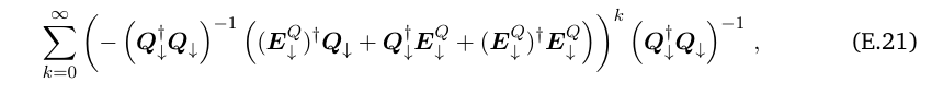
\ Claim E.4 (Neumann series truncation). It holds that
\
\ Proof. For the Neumann series term in Eq. (E.10):
\
\ we first bound the middle bracket:
\
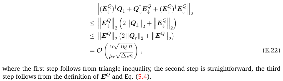
\ The first-order term (i.e., k = 1) in Eq. (E.21) can be approximated as follows:
\
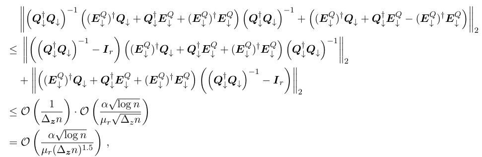
\ where the first step follows from triangle inequality, the second step follows from Eq. (E.18) and Eq. (E.22), and the last step is by direct calculation.
\ By a similar calculation, we can show that the second-order term (i.e., k = 2) in Eq. (E.21) can be approximated by
\
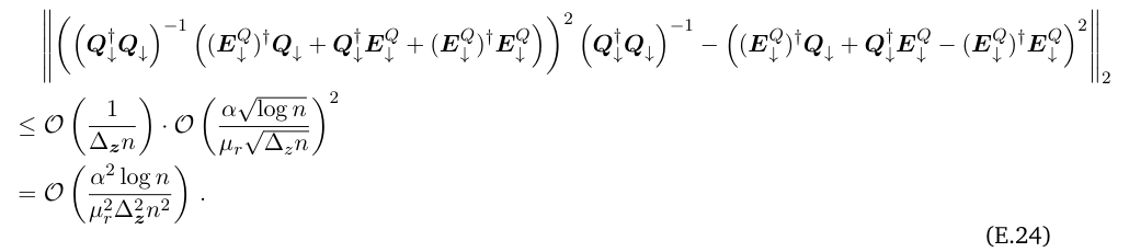
\ Indeed, this term can be further simplified:
\
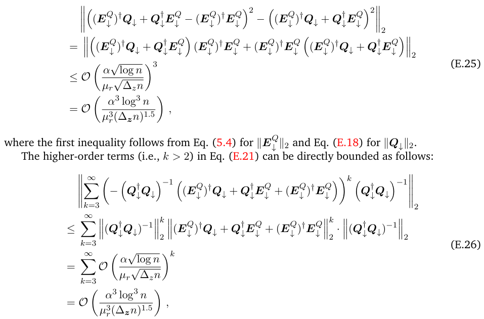
\ where the first step follows from triangle inequality, the second step follows from Eq. (E.18) and Eq. (E.22), and the last step follows from the geometric summation.
\ Combining Eq. (E.23) to Eq. (E.26) together, we get that
\
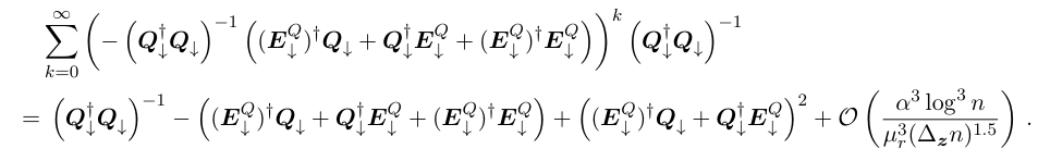
\ The claim is then proved.
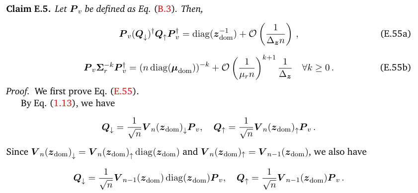
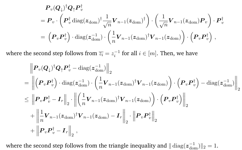
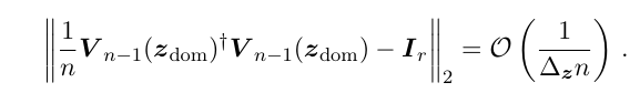
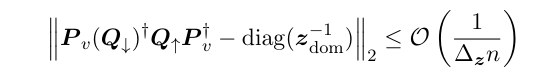
E.3 Proofs for Step 3: Error cancellation in the Taylor expansionE.3.1 Establishing the first equation in Eq. (5.10)
\
\ Proof. In this proof, we often use the following observations:
\
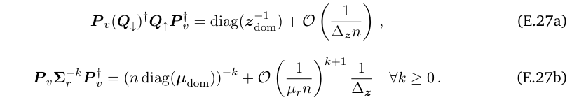
\ They are proved in Claim E.5.
\
\ we have
\
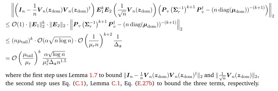
\ where the third step uses Lemma 1.7 for the first term, Eq. (C.1) for the second term, Lemma C.1 for the third term, Eq. (1.14) for the fifth and seventh terms, Eq. (B.2) for the sixth term. Thus,
\
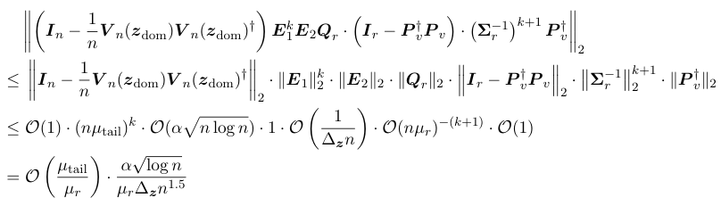
\ To bound the second term in the above equation, for any k ≥ 0, we have
\
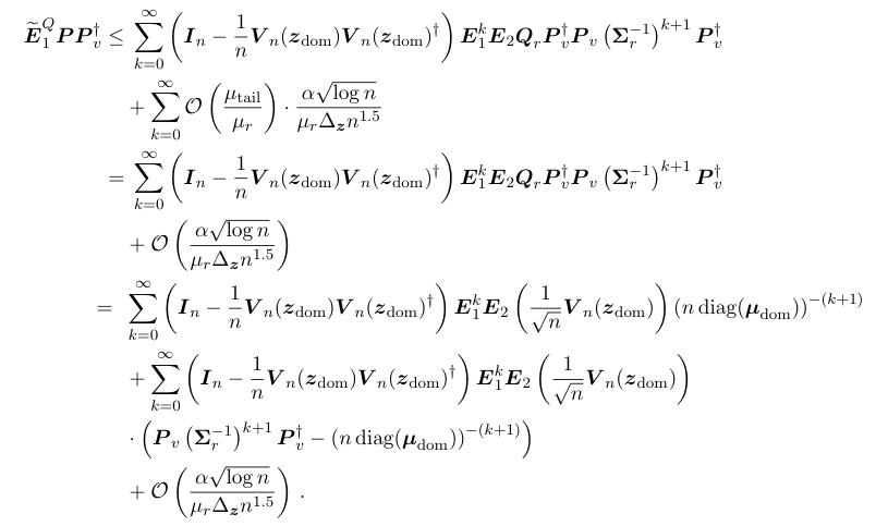
\ Therefore, we obtain that
\
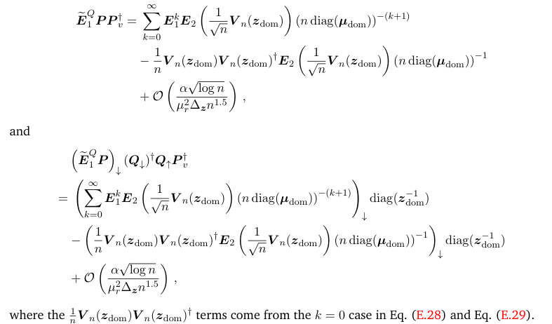
\ Similarly, we also have
\
\
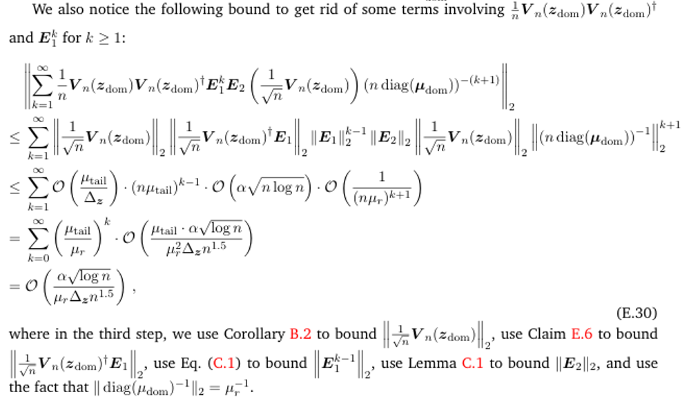
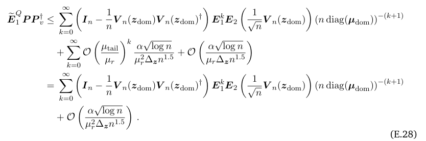
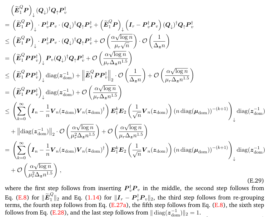
\ Plugging Eq. (E.30) into Eq. (E.28) and Eq. (E.29), we have
\
\ The proof of the lemma is completed.
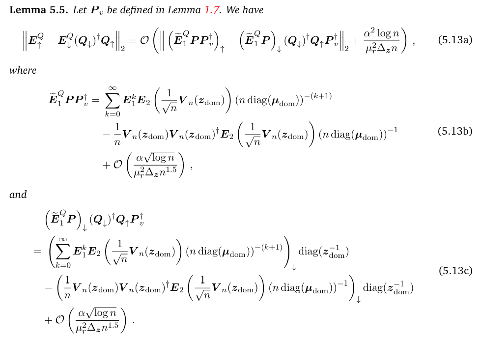
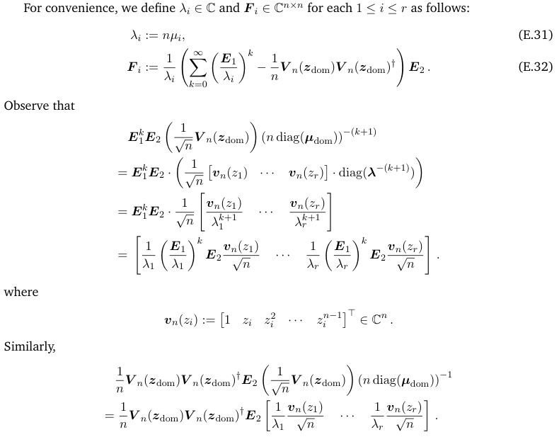
\ Lemma 5.6.
\

\ Proof. We analyze Eq. (5.13b) and Eq. (5.13c) column-by-column.
\
\ Combining the above two equations together and summing over k, we obtain that
\
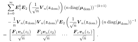
\ By Eq. (5.13b) and Eq. (5.13c), we have
\
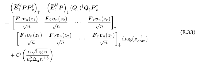
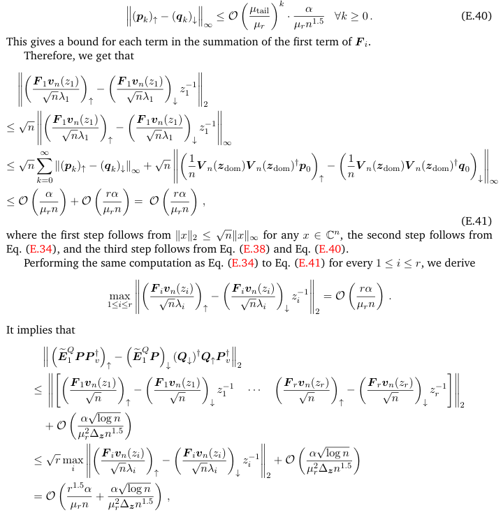
\ Without loss of generality, we only consider the first column of Eq. (E.33):
\
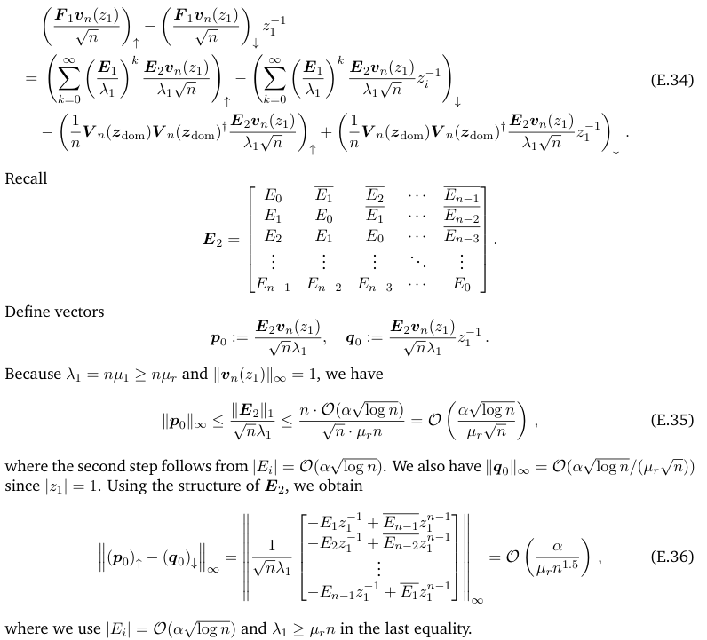
\
\ where the second step follows from the Toeplize structure of the matrix. Therefore, by triangle inequality,
\
\ where the second step follows from Eq. (E.35)-Eq. (E.37).
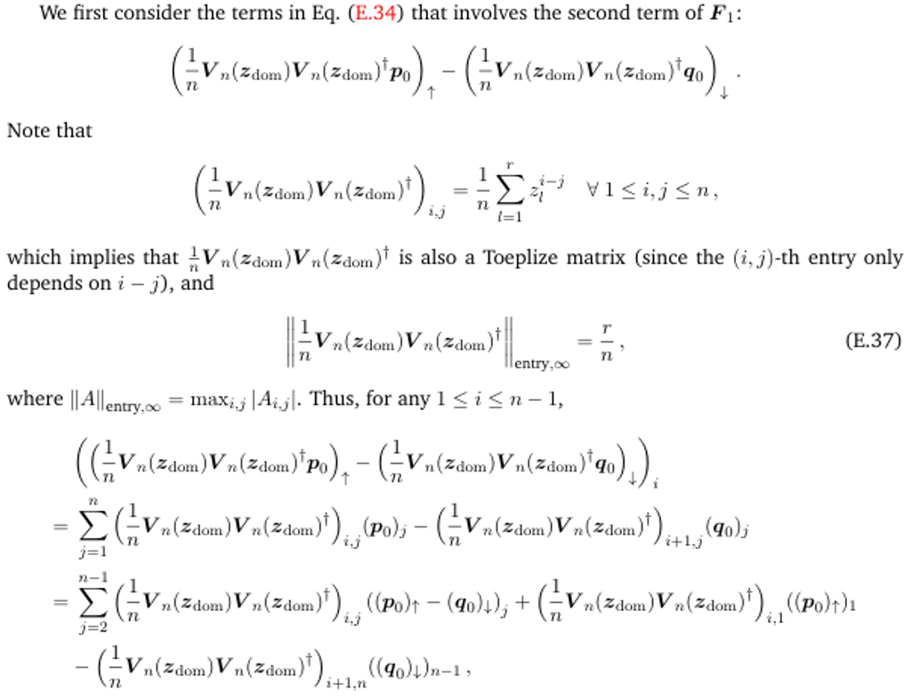
\ Now, we consider the first term of F1. Define
\
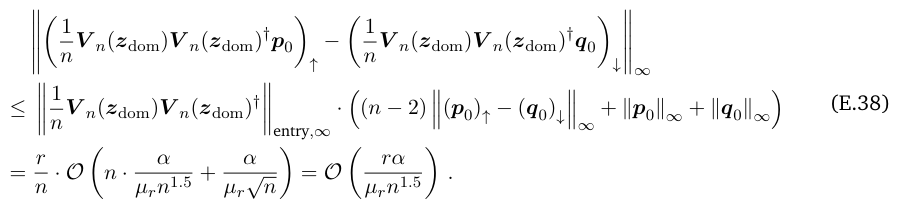
\ where the second step follows from Eq. (E.39). The above two equations imply that
\
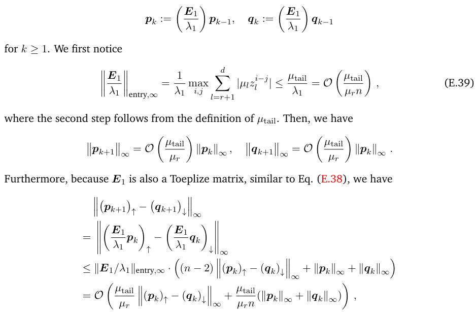
\ Plugging in the values of k = 0 in Eq. (E.35) and Eq. (E.36), we obtain for any k > 0
\
\ which implies that
\
\
\ Thus, we obtain that
\
\
\ Combining Eq. (E.44) and Eq. (E.45) together, the lemma is proved.
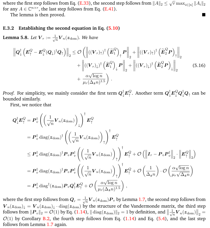
\ Lemma 5.9.
\
\
\
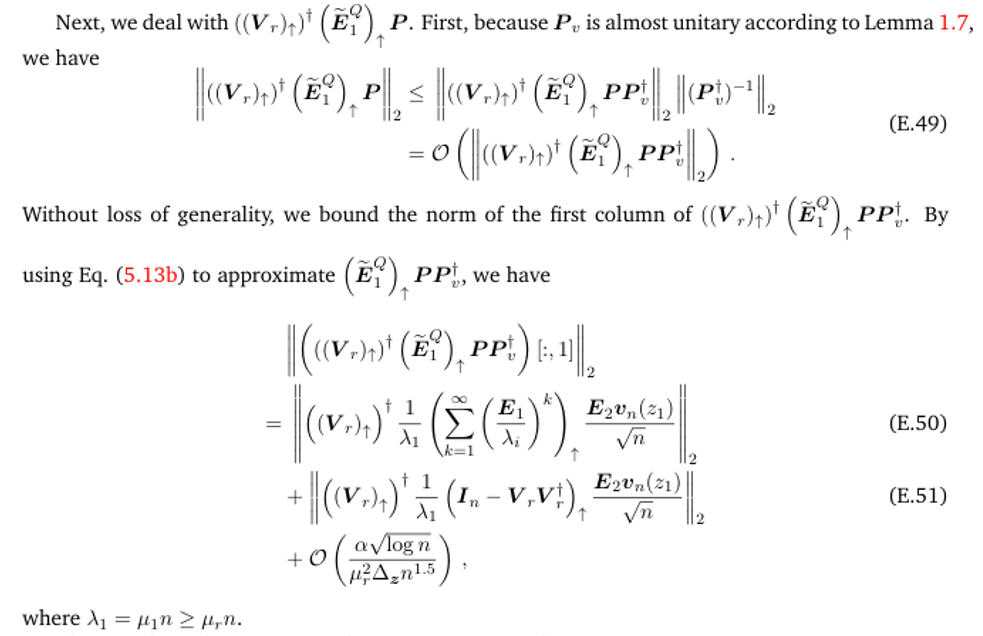
\ Then, we bound Eq. (E.50) and Eq. (E.51) separately.
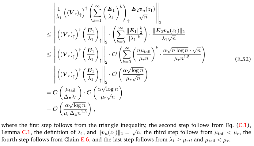
\ For Eq. (E.50), we have
\
\ For Eq. (E.51), we notice that
\
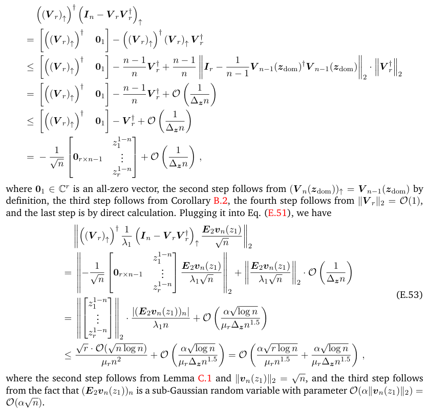
\ Hence, combining Eq. (E.52) and Eq. (E.53) together, we obtain
\
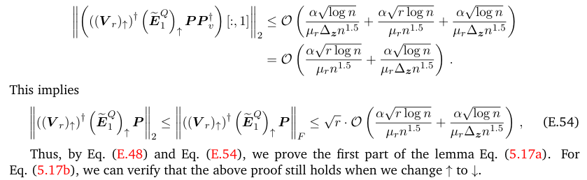
\ Therefore, we complete the proof of the lemma.
\ E.3.3 Technical claims
\
\ Thus, LHS of Eq. (E.55) can be expressed as:
\
\ By a slightly modified proof of Corollary B.2, it is easy to show that
\
\ Together with Lemma 1.7, we obtain that
\
\ which proves the first part of the claim.
\ Next, we prove Eq. (E.55b).
\ When k = 0, Eq. (E.55b) becomes
\
\ which follows from Lemma 1.7.
\ When k ≥ 1, we have
\
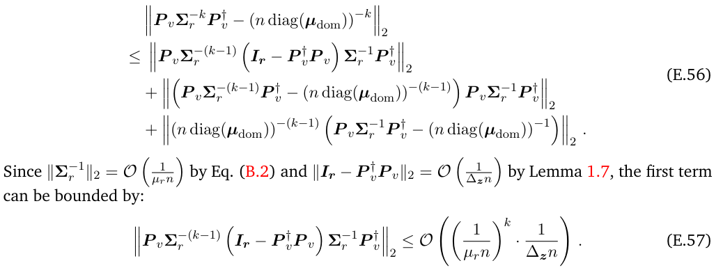
\ Similarly, the second term can be bounded by:
\
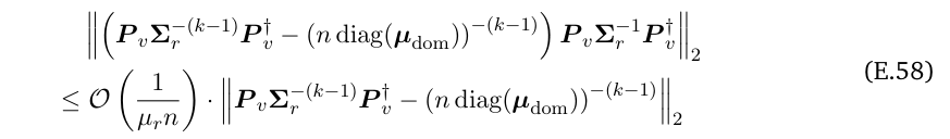
\ The third term can be bounded by:
\
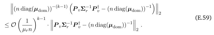
\ Hence, to prove Eq. (E.55b), it suffices to bound
\
\
\ where the first step follows from Lemma 1.7, and the second step follows from Eq. (1.14). Combining the above three equations together, we obtain
\
\ where the second step follows from using Corollary B.3. This proves the k = 1 case of Eq. (E.55b).
\ Finally, by induction Eqs. (E.56) to (E.59), we can prove that for any k ≥ 2,
\
\ This concludes the proof of Eq. (E.55b).
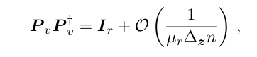
\ Claim E.6.
\

\ The claim then follows.
\
:::info This paper is available on arxiv under CC BY 4.0 DEED license.
:::
:::info Authors:
(1) Zhiyan Ding, Department of Mathematics, University of California, Berkeley;
(2) Ethan N. Epperly, Department of Computing and Mathematical Sciences, California Institute of Technology, Pasadena, CA, USA;
(3) Lin Lin, Department of Mathematics, University of California, Berkeley, Applied Mathematics and Computational Research Division, Lawrence Berkeley National Laboratory, and Challenge Institute for Quantum Computation, University of California, Berkeley;
(4) Ruizhe Zhang, Simons Institute for the Theory of Computing.
:::
\