Detailed Experimentation and Comparisons for Continual Learning Methods

:::info Authors:

(1) Sebastian Dziadzio, University of Tübingen ([email protected]);

(2) Çagatay Yıldız, University of Tübingen;

(3) Gido M. van de Ven, KU Leuven;

(4) Tomasz Trzcinski, IDEAS NCBR, Warsaw University of Technology, Tooploox;

(5) Tinne Tuytelaars, KU Leuven;

(6) Matthias Bethge, University of Tübingen.

:::

Table of Links

Abstract and 1. Introduction

2. Two problems with the current approach to class-incremental continual learning

3. Methods and 3.1. Infinite dSprites

3.2. Disentangled learning

4. Related work

4.1. Continual learning and 4.2. Benchmarking continual learning

5. Experiments

5.1. Regularization methods and 5.2. Replay-based methods

5.3. Do we need equivariance?

5.4. One-shot generalization and 5.5. Open-set classification

5.6. Online vs. offline

Conclusion, Acknowledgments and References

Supplementary Material

Supplementary Material 1. Experiment details

All models employ the same ResNet-18 [9] backbone and are trained using the Adam optimizer [14] with default PyTorch [27] parameter values (λ = 0.001, β1 = 0.9, β2 = 0.999). For our method we always report the average test accuracy over 5 runs with 5 epochs per task. For other methods, due to computational constraints, we only report the accuracy of a single run.

1.1. Regularization methods

We ran a grid search to set the loss balance weight λo in LwF [18] and the strength parameter c in SI [39], but found the choice of hyperparameter did not influence the result. For the run shown in Figure Fig. 4, we used λo = 0.1 and c = 0.1.

1.2. Replay methods

For the experiments presented in the main text, we use a modified version of experience replay, inspired by the approach of GDumb [28]. At the beginning of each task t, we add all the training data from the current task to the buffer. If the buffer is full, we employ reservoir sampling so that the memory buffer contains an equal number of examples of every class seen so far, including the classes in task t. We then train the model on the memory buffer until convergence and report test accuracy.

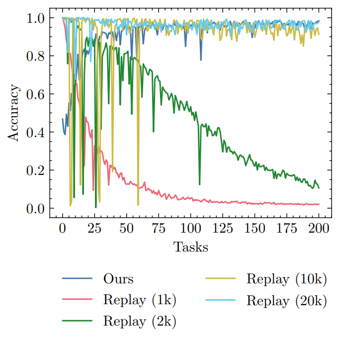
\ Here we present results for a different rehearsal approach. For each task t, we extend every mini-batch of the training set with an equal number of samples chosen randomly (with replacement) from the buffer. We train the model for five epochs per task. Figure 1 shows a comparison of this training protocol to our method. Surprisingly, this way of doing replay yields better test set accuracy than the replay baseline we used in the main text, despite putting a disproportionate weight on the current task.

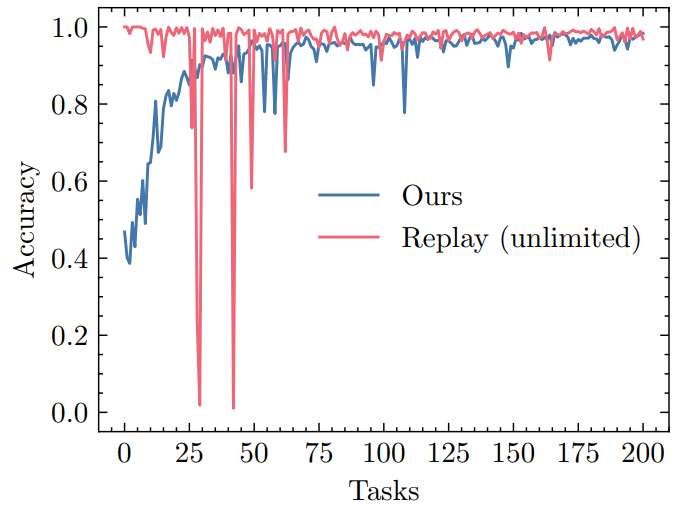
\ Figure 2 shows a comparison of our method to experience replay with no limit on the buffer size. Here we also mix the samples from the current task with randomly chosen buffer samples and train for five epochs per task.

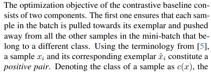
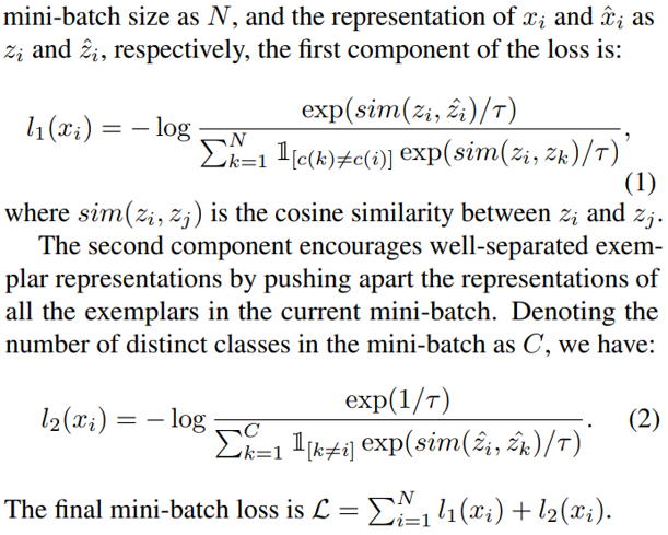
1.3. Contrastive baseline

\

\

\

\

:::info This paper is available on arxiv under CC 4.0 license.

:::

\