and the distribution of digital products.
The Calvo Wage Phillips Curve and Labor Market Imperfections
:::info Author:
(1) David Staines.
:::
Table of Links4 Calvo Framework and 4.1 Household’s Problem
4.3 Household Equilibrium Conditions
4.5 Nominal Equilibrium Conditions
4.6 Real Equilibrium Conditions and 4.7 Shocks
5.2 Persistence and Policy Puzzles
6 Stochastic Equilibrium and 6.1 Ergodic Theory and Random Dynamical Systems
7 General Linearized Phillips Curve
8 Existence Results and 8.1 Main Results
9.2 Algebraic Aspects (I) Singularities and Covers
9.3 Algebraic Aspects (II) Homology
9.4 Algebraic Aspects (III) Schemes
9.5 Wider Economic Interpretations
10 Econometric and Theoretical Implications and 10.1 Identification and Trade-offs
10.4 Microeconomic Interpretation
\ Appendices
A Proof of Theorem 2 and A.1 Proof of Part (i)
B Proofs from Section 4 and B.1 Individual Product Demand (4.2)
B.2 Flexible Price Equilibrium and ZINSS (4.4)
B.4 Cost Minimization (4.6) and (10.4)
C Proofs from Section 5, and C.1 Puzzles, Policy and Persistence
D Stochastic Equilibrium and D.1 Non-Stochastic Equilibrium
D.2 Profits and Long-Run Growth
E Slopes and Eigenvalues and E.1 Slope Coefficients
E.4 Rouche’s Theorem Conditions
F Abstract Algebra and F.1 Homology Groups
F.4 Marginal Costs and Inflation
G Further Keynesian Models and G.1 Taylor Pricing
G.3 Unconventional Policy Settings
H Empirical Robustness and H.1 Parameter Selection
I Additional Evidence and I.1 Other Structural Parameters
I.3 Trend Inflation Volatility
G.2 Calvo Wage Phillips CurveThis subsection shows a wage Phillips curve problem and how results of Theorem 8 apply. First, I introduce imperfect competition into the labor market before showing that the associated resetting problem is analogous to that of the price Phillips curve (26)-(31).
\ G.2.1 Labor Unions
\ In the benchmark model of Section 4 the labor market is perfectly competitive. To generate wage rigidity, we need to introduce imperfect substitutability between wage setters. The easiest way to achieve this is to introduce unions, which combine different types of labor into a composite labor service, that is leased to firms at a wage rate W. The aggregation is as follows
\
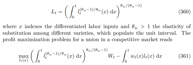
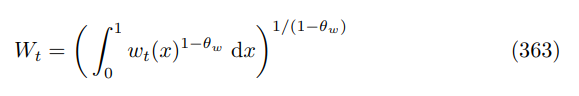
\ This yields the labor demand system
\
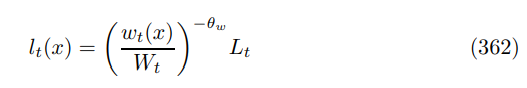
\ and the wage index
\
\ G.2.2 Optimization Problem
\ The union sets wages to maximize the welfare of its members. It gets to reset wages with probability αw each period. The problem can be written as follows
\
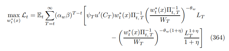
\ where I have used the functional form for the disutility of labor. The first order condition is
\
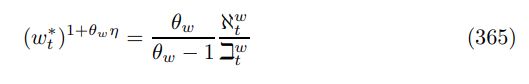
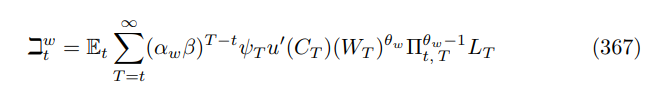
\ with
\
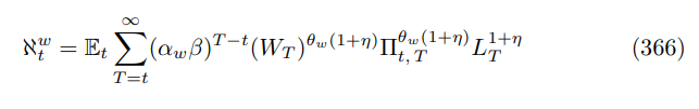
\
\ Optimal reset wage can be viewed as a generalized weighted mean of flexible wages, according to Proposition 27 since
\
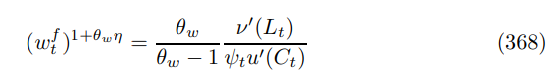
\ which are set as a mark up over the marginal rate of substitution between labor and leisure, which is decreasing in the substitutability between labor varieties. Aggregate wages evolve according to
\
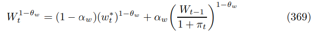
\ The difference with the price level construction equation is that we are using real wages as opposed to nominal prices. The final and crucial step is to expand out the recursions (366) and (367)
\
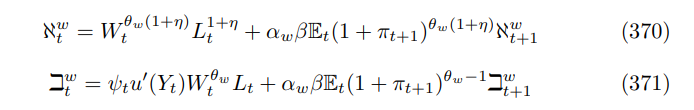
\ Linearizing these equations at ZINSS, it is clear that a common root in the lag polynomials will arise with
\
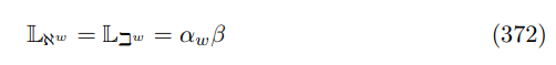
\ This confirms we can apply Theorem 7 and conclude a bifurcation invalidates the linear approximations at ZINSS, without having to go through a detailed solution. Moreover, this analysis extends to larger models typically used in central banks, which feature both price and wage rigidity, like Christiano et al. [2005] and Smets and Wouters [2007].
\
:::info This paper is available on arxiv under CC 4.0 license.
:::
\