Beyond Text Embeddings: Addressing the Gaps in RAG Applications for Structured Data Queries

\ Everyone loves text embedding models, and for good reason: They excel at encoding unstructured text, making it easier to discover semantically similar content. It’s no surprise that they form the backbone of most RAG applications, especially with the current emphasis on encoding and retrieving relevant information from documents and other textual resources. However, there are clear examples of questions one might ask where the text embedding approach to RAG applications falls short and delivers incorrect information.

\ As mentioned, text embeddings are great at encoding unstructured text. On the other hand, they aren’t that great at dealing with structured information and operations such as filtering, sorting, or aggregations. Imagine a simple question like:

\

What is the highest-rated movie released in 2024?

\ To answer this question, we must first filter by release year, followed by sorting by rating. We’ll examine how a naive approach with text embeddings performs and then demonstrate how to deal with such questions. This blog post showcases that when dealing with structured data operations such as filtering, sorting, or aggregating, you need to use other tools that provide structure such as knowledge graphs.

\ The code is available on GitHub.

Environment Setup

For this blog post, we’ll use the recommendations project in Neo4j Sandbox. The recommendations project uses the MovieLens dataset, which contains movies, actors, ratings, and more information.

\

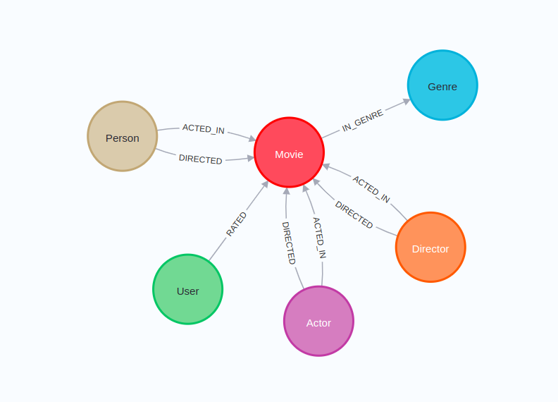
\ The following code will instantiate a LangChain wrapper to connect to Neo4j Database:

\

os.environ["NEO4J_URI"] = "bolt://44.204.178.84:7687" os.environ["NEO4J_USERNAME"] = "neo4j" os.environ["NEO4J_PASSWORD"] = "minimums-triangle-saving" graph = Neo4jGraph(refresh_schema=False)

\ Additionally, you will require an OpenAI API key that you pass in the following code:

\

os.environ["OPENAI_API_KEY"] = getpass.getpass("OpenAI API Key:")

\ The database contains 10,000 movies, but text embeddings are not yet stored. To avoid calculating embeddings for all of them, we’ll tag the 1,000 top-rated films with a secondary label called Target:

\

graph.query(""" MATCH (m:Movie) WHERE m.imdbRating IS NOT NULL WITH m ORDER BY m.imdbRating DESC LIMIT 1000 SET m:Target """) Calculating and Storing Text Embeddings

Deciding what to embed is an important consideration. Since we’ll be demonstrating filtering by year and sorting by rating, it wouldn’t be fair to exclude those details from the embedded text. That’s why I chose to capture the release year, rating, title, and description of each movie.

\ Here is an example of text we will embed for The Wolf of Wall Street movie:

\

plot: Based on the true story of Jordan Belfort, from his rise to a wealthy stock-broker living the high life to his fall involving crime, corruption and the federal government. title: Wolf of Wall Street, The year: 2013 imdbRating: 8.2

\ You might say this is not a good approach to embedding structured data, and I wouldn’t argue since I don’t know the best approach. Maybe instead of key-value items, we should convert them to text or something. Let me know if you have some ideas about what might work better.

\ The Neo4j Vector object in LangChain has a convenient method fromexistinggraphwhere you can select which text properties should be encoded:

\

embedding = OpenAIEmbeddings(model="text-embedding-3-small") neo4j_vector = Neo4jVector.from_existing_graph( embedding=embedding, index_name="movies", node_label="Target", text_node_properties=["plot", "title", "year", "imdbRating"], embedding_node_property="embedding", )

\ In this example, we use OpenAI’s text-embedding-3-small model for embedding generation. We initialize the Neo4jVector object using the fromexistinggraph method. The nodelabel parameter filters the nodes to be encoded, specifically those labeled Target. The textnodeproperties parameter defines the node properties to be embedded, including plot, title, year, and imdbRating. Finally, the embeddingnode_property defines the property where the generated embeddings will be stored, designated as embedding.

The Naive Approach

Let’s start by trying to find a movie based on its plot or description:

\

pretty_print( neo4j_vector.similarity_search( "What is a movie where a little boy meets his hero?" ) )

\ Results:

\

plot: A young boy befriends a giant robot from outer space that a paranoid government agent wants to destroy. title: Iron Giant, The year: 1999 imdbRating: 8.0 plot: After the death of a friend, a writer recounts a boyhood journey to find the body of a missing boy. title: Stand by Me year: 1986 imdbRating: 8.1 plot: A young, naive boy sets out alone on the road to find his wayward mother. Soon he finds an unlikely protector in a crotchety man and the two have a series of unexpected adventures along the way. title: Kikujiro (Kikujirô no natsu) year: 1999 imdbRating: 7.9 plot: While home sick in bed, a young boy's grandfather reads him a story called The Princess Bride. title: Princess Bride, The year: 1987 imdbRating: 8.1

\ The results seem pretty solid overall. There’s consistently a little boy involved, though I’m not sure if he always meets his hero. Then again, the dataset only includes 1,000 movies, so the options are somewhat limited.

\ Now let’s try a query that requires some basic filtering:

\

pretty_print( neo4j_vector.similarity_search( "Which movies are from year 2016?" ) )

\ Results:

\

plot: Six short stories that explore the extremities of human behavior involving people in distress. title: Wild Tales year: 2014 imdbRating: 8.1 plot: A young man who survives a disaster at sea is hurtled into an epic journey of adventure and discovery. While cast away, he forms an unexpected connection with another survivor: a fearsome Bengal tiger. title: Life of Pi year: 2012 imdbRating: 8.0 plot: Based on the true story of Jordan Belfort, from his rise to a wealthy stock-broker living the high life to his fall involving crime, corruption and the federal government. title: Wolf of Wall Street, The year: 2013 imdbRating: 8.2 plot: After young Riley is uprooted from her Midwest life and moved to San Francisco, her emotions - Joy, Fear, Anger, Disgust and Sadness - conflict on how best to navigate a new city, house, and school. title: Inside Out year: 2015 imdbRating: 8.3

\ It’s funny, but not a single movie from 2016 was selected. Maybe we could get better results with different text preparation for encoding. However, text embeddings aren’t applicable here since we’re dealing with a simple structured data operation where we need to filter documents or, in this example, movies based on a metadata property. Metadata filtering is a well-established technique often employed to enhance the accuracy of RAG systems.

\ The next query we’ll try requires a bit of sorting:

\

pretty_print( neo4j_vector.similarity_search("Which movie has the highest imdb score?") )

\ Results:

\

plot: A silent film production company and cast make a difficult transition to sound. title: Singin' in the Rain year: 1952 imdbRating: 8.3 plot: A film about the greatest pre-Woodstock rock music festival. title: Monterey Pop year: 1968 imdbRating: 8.1 plot: This movie documents the Apollo missions perhaps the most definitively of any movie under two hours. Al Reinert watched all the footage shot during the missions--over 6,000,000 feet of it, ... title: For All Mankind year: 1989 imdbRating: 8.2 plot: An unscrupulous movie producer uses an actress, a director and a writer to achieve success. title: Bad and the Beautiful, The year: 1952 imdbRating: 7.9

\ If you’re familiar with IMDb ratings, you know there are plenty of movies scoring above 8.3. The highest-rated title in our database is actually a series — Band of Brothers — with an impressive 9.6 rating. Once again, text embeddings perform poorly when it comes to sorting results.

\ Let’s also evaluate a question that requires some sort of aggregation:

\

pretty_print(neo4j_vector.similarity_search("How many movies are there?"))

\ Results:

\

plot: Ten television drama films, each one based on one of the Ten Commandments. title: Decalogue, The (Dekalog) year: 1989 imdbRating: 9.2 plot: A documentary which challenges former Indonesian death-squad leaders to reenact their mass-killings in whichever cinematic genres they wish, including classic Hollywood crime scenarios and lavish musical numbers. title: Act of Killing, The year: 2012 imdbRating: 8.2 plot: A meek Hobbit and eight companions set out on a journey to destroy the One Ring and the Dark Lord Sauron. title: Lord of the Rings: The Fellowship of the Ring, The year: 2001 imdbRating: 8.8 plot: While Frodo and Sam edge closer to Mordor with the help of the shifty Gollum, the divided fellowship makes a stand against Sauron's new ally, Saruman, and his hordes of Isengard. title: Lord of the Rings: The Two Towers, The year: 2002 imdbRating: 8.7

\ The results are definitely not helpful here because we get four random movies returned. It’s virtually impossible to get from these random four movies a conclusion that there are a total of 1,000 movies we tagged and embedded for this example.

\ So what’s the solution? It’s straightforward: Questions involving structured operations like filtering, sorting, and aggregation need tools designed to operate with structured data.

Tools for Structured Data

At the moment, it seems that most people think about the text2query approach, where an LLM generates a database query to interact with a database based on the provided question and schema. For Neo4j, this is text2cypher, but there is also text2sql for SQL databases. However, it turns out in practice that it isn’t reliable and not robust enough for production use.

\

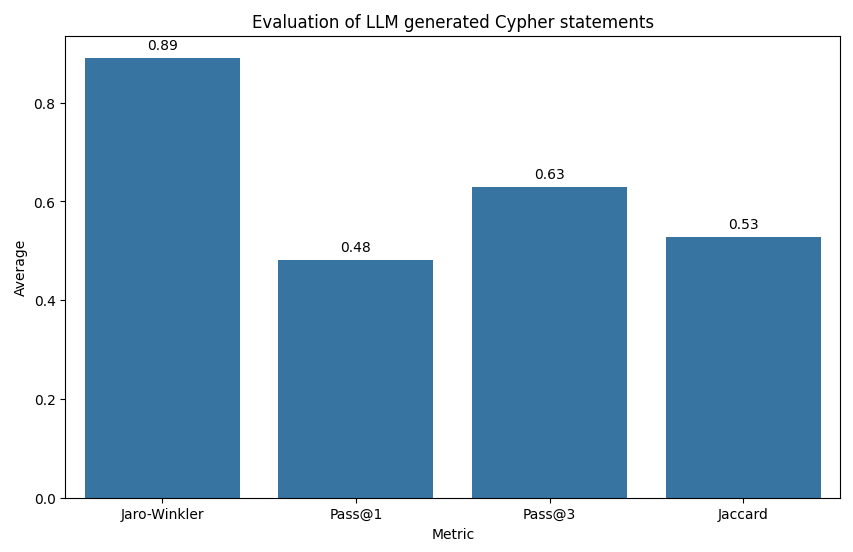
Cypher statement generation evaluation. Taken from my blog post about Cypher evaluation.

\ You can use techniques like chain of thought, few-shot examples, or fine-tuning, but achieving high accuracy remains nearly impossible at this stage. The text2query approach works well for simple questions on straightforward database schemas, but that’s not the reality of production environments. To address this, we shift the complexity of generating database queries away from an LLM and treat it as a code problem where we generate database queries deterministically based on function inputs. The advantage is significantly improved robustness, though it comes at the cost of reduced flexibility. It’s better to narrow the scope of the RAG application and answer those questions accurately, rather than attempt to answer everything but do so inaccurately.

\ Since we are generating database queries — in this case, Cypher statements — based on function inputs, we can leverage the tool capabilities of LLMs. In this process, the LLM populates the relevant parameters based on user input, while the function handles retrieving the necessary information. For this demonstration, we’ll first implement two tools: one for counting movies and another for listing them, and then create an LLM agent using LangGraph.

Tool for Counting Movies

We begin by implementing a tool for counting movies based on predefined filters. First, we have to define what those filters are and describe to an LLM when and how to use them:

\

class MovieCountInput(BaseModel): min_year: Optional[int] = Field( description="Minimum release year of the movies" ) max_year: Optional[int] = Field( description="Maximum release year of the movies" ) min_rating: Optional[float] = Field(description="Minimum imdb rating") grouping_key: Optional[str] = Field( description="The key to group by the aggregation", enum=["year"] )

\ LangChain offers several ways to define function inputs, but I prefer the Pydantic approach. In this example, we have three filters available to refine movie results: minyear, maxyear, and minrating. These filters are based on structured data and are optional, as the user may choose to include any, all, or none of them. Additionally, we’ve introduced a groupingkey input that tells the function whether to group the count by a specific property. In this case, the only supported grouping is by year, as defined in the enumsection.

\ Now let’s define the actual function:

\

@tool("movie-count", args_schema=MovieCountInput) def movie_count( min_year: Optional[int], max_year: Optional[int], min_rating: Optional[float], grouping_key: Optional[str], ) -> List[Dict]: """Calculate the count of movies based on particular filters""" filters = [ ("t.year >= $min_year", min_year), ("t.year <= $max_year", max_year), ("t.imdbRating >= $min_rating", min_rating), ] # Create the parameters dynamically from function inputs params = { extract_param_name(condition): value for condition, value in filters if value is not None } where_clause = " AND ".join( [condition for condition, value in filters if value is not None] ) cypher_statement = "MATCH (t:Target) " if where_clause: cypher_statement += f"WHERE {where_clause} " return_clause = ( f"t.`{grouping_key}`, count(t) AS movie_count" if grouping_key else "count(t) AS movie_count" ) cypher_statement += f"RETURN {return_clause}" print(cypher_statement) # Debugging output return graph.query(cypher_statement, params=params)

\ The movie_count function generates a Cypher query to count movies based on optional filters and grouping key. It begins by defining a list of filters with corresponding values provided as arguments. The filters are used to dynamically build the WHERE clause, which is responsible for applying the specified filtering conditions in the Cypher statement, including only those conditions where values are not None.

\ The RETURN clause of the Cypher query is then constructed, either grouping by the provided grouping_key or simply counting the total number of movies. Finally, the function executes the query and returns the results.

\ The function can be extended with more arguments and more involved logic as needed, but it’s important to ensure that it remains clear so that an LLM can call it correctly and accurately.

Tool for Listing Movies

Again, we have to start by defining the arguments of the function:

\

class MovieListInput(BaseModel): sort_by: str = Field( description="How to sort movies, can be one of either latest, rating", enum=["latest", "rating"], ) k: Optional[int] = Field(description="Number of movies to return") description: Optional[str] = Field(description="Description of the movies") min_year: Optional[int] = Field( description="Minimum release year of the movies" ) max_year: Optional[int] = Field( description="Maximum release year of the movies" ) min_rating: Optional[float] = Field(description="Minimum imdb rating")

\ We keep the same three filters as in the movie count function but add the description argument. This argument lets us search and list movies based on their plot using vector similarity search. Just because we’re using structured tools and filters doesn’t mean we can’t incorporate text embedding and vector search methods. Since we don’t want to return all movies most of the time, we include an optional k input with a default value. Additionally, for listing, we want to sort the movies to return only the most relevant ones. In this case, we can sort them by rating or release year.

\ Let’s implement the function:

\

@tool("movie-list", args_schema=MovieListInput) def movie_list( sort_by: str = "rating", k : int = 4, description: Optional[str] = None, min_year: Optional[int] = None, max_year: Optional[int] = None, min_rating: Optional[float] = None, ) -> List[Dict]: """List movies based on particular filters""" # Handle vector-only search when no prefiltering is applied if description and not min_year and not max_year and not min_rating: return neo4j_vector.similarity_search(description, k=k) filters = [ ("t.year >= $min_year", min_year), ("t.year <= $max_year", max_year), ("t.imdbRating >= $min_rating", min_rating), ] # Create parameters dynamically from function arguments params = { key.split("$")[1]: value for key, value in filters if value is not None } where_clause = " AND ".join( [condition for condition, value in filters if value is not None] ) cypher_statement = "MATCH (t:Target) " if where_clause: cypher_statement += f"WHERE {where_clause} " # Add the return clause with sorting cypher_statement += " RETURN t.title AS title, t.year AS year, t.imdbRating AS rating ORDER BY " # Handle sorting logic based on description or other criteria if description: cypher_statement += ( "vector.similarity.cosine(t.embedding, $embedding) DESC " ) params["embedding"] = embedding.embed_query(description) elif sort_by == "rating": cypher_statement += "t.imdbRating DESC " else: # sort by latest year cypher_statement += "t.year DESC " cypher_statement += " LIMIT toInteger($limit)" params["limit"] = k or 4 print(cypher_statement) # Debugging output data = graph.query(cypher_statement, params=params) return data

\ This function retrieves a list of movies based on multiple optional filters: description, year range, minimum rating, and sorting preferences. If only a description is given with no other filters, it performs a vector index similarity search to find relevant movies. When additional filters are applied, the function constructs a Cypher query to match movies based on the specified criteria, such as release year and IMDb rating, combining them with an optional description-based similarity. The results are then sorted by either the similarity score, IMDb rating, or year, and limited to k movies.

Putting It All Together as a LangGraph Agent

We will implement a straightforward ReAct agent using LangGraph.

\

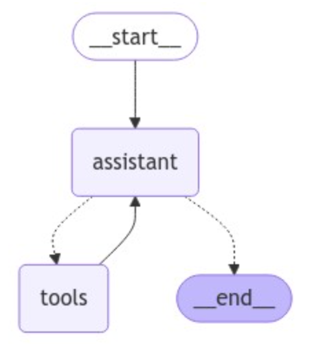
\ The agent consists of an LLM and tools step. As we interact with the agent, we’ll first call the LLM to decide if we should use tools. Then we’ll run a loop:

\

1. If the agent said to take an action (i.e., call tool), we’ll run the tools and pass the results back to the agent.
2. If the agent did not ask to run tools, we’ll finish (respond to the user).

\ The code implementation is as straightforward as it gets. First we bind the tools to the LLM and define the assistant step:

\

llm = ChatOpenAI(model='gpt-4-turbo') tools = [movie_count, movie_list] llm_with_tools = llm.bind_tools(tools) # System message sys_msg = SystemMessage(content="You are a helpful assistant tasked with finding and explaining relevant information about movies.") # Node def assistant(state: MessagesState): return {"messages": [llm_with_tools.invoke([sys_msg] + state["messages"])]}

\ Next we define the LangGraph flow:

\

# Graph builder = StateGraph(MessagesState) # Define nodes: these do the work builder.add_node("assistant", assistant) builder.add_node("tools", ToolNode(tools)) # Define edges: these determine how the control flow moves builder.add_edge(START, "assistant") builder.add_conditional_edges( "assistant", # If the latest message (result) from assistant is a tool call -> tools_condition routes to tools # If the latest message (result) from assistant is a not a tool call -> tools_condition routes to END tools_condition, ) builder.add_edge("tools", "assistant") react_graph = builder.compile()

\ We define two nodes in the LangGraph and link them with a conditional edge. If a tool is called, the flow is directed to the tools; otherwise, the results are sent back to the user.

\ Let’s now test our agent:

\

messages = [ HumanMessage( content="What are the some movies about a girl meeting her hero?" ) ] messages = react_graph.invoke({"messages": messages}) for m in messages["messages"]: m.pretty_print()

\ Results:

\

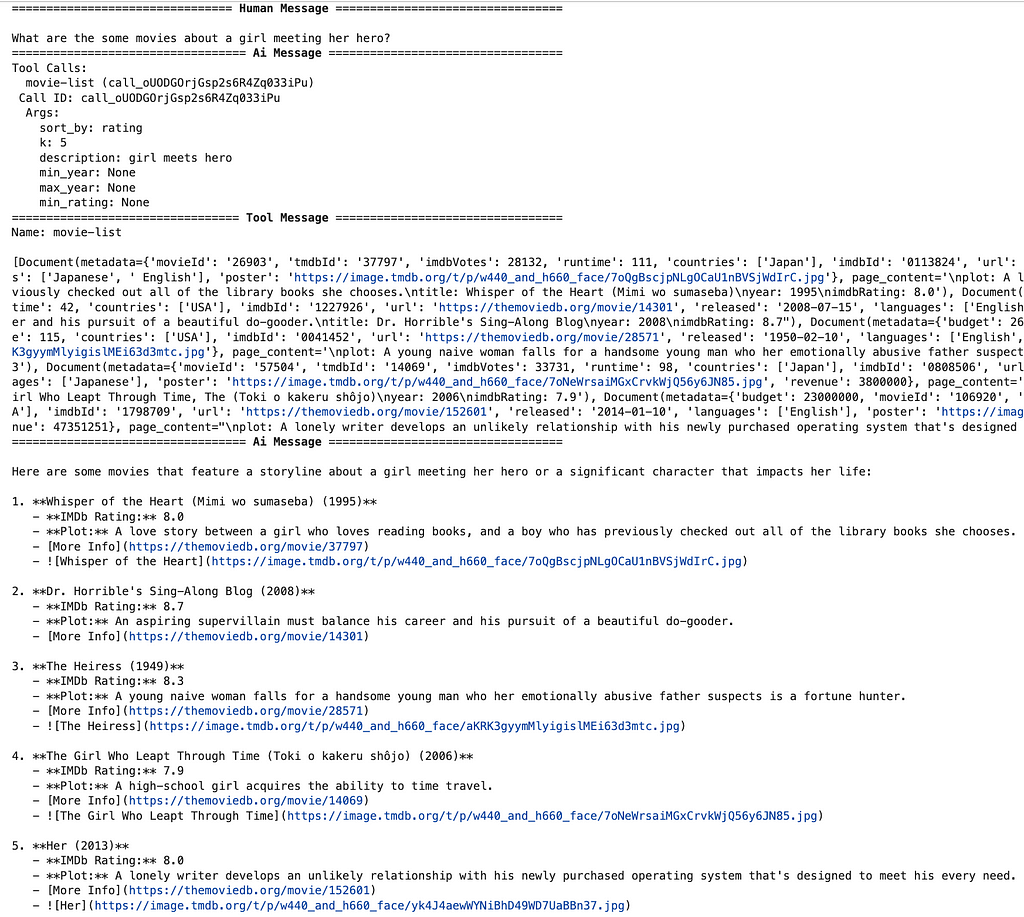
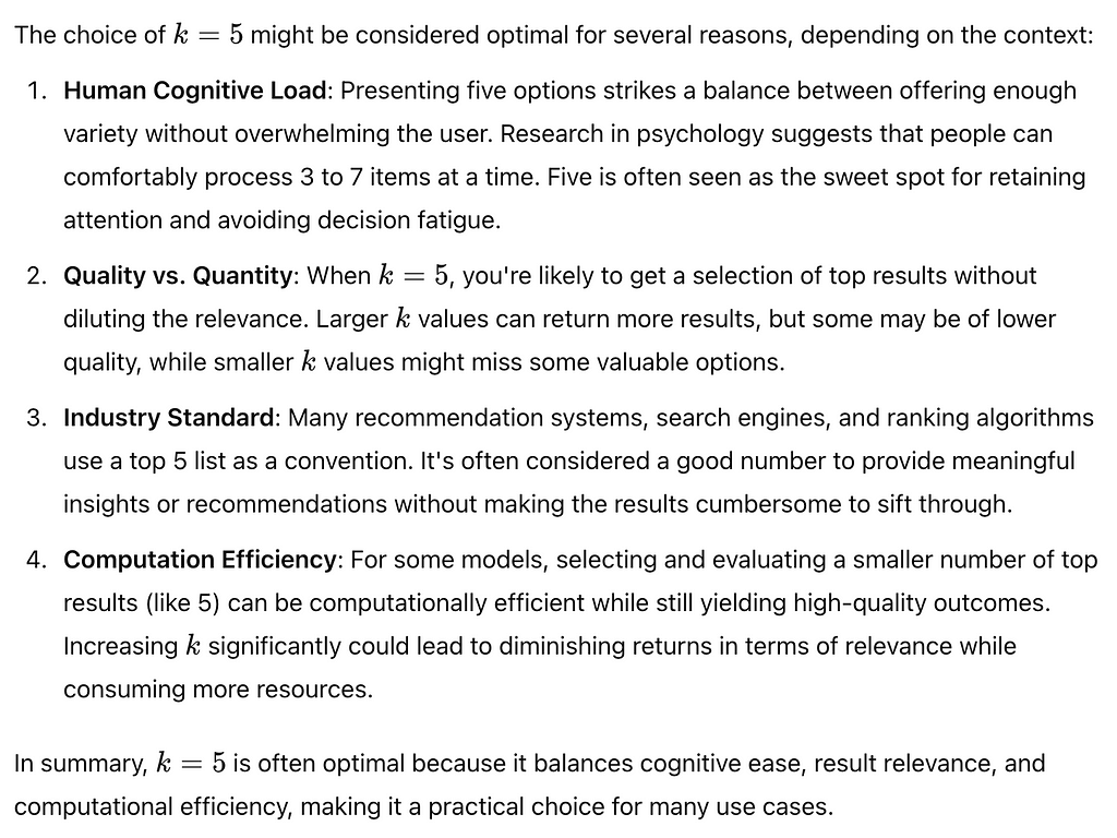
\ In the first step, the agent chooses to use the movie-list tool with the appropriate descriptionparameter. It’s unclear why it selects a kvalue of 5, but it seems to favor that number. The tool returns the top five most relevant movies based on the plot, and the LLM simply summarizes them for the user at the end.

\ If we ask ChatGPT why it likes k value of 5, we get the following response.

\

\ Next, let’s ask a slightly more complex question that requires metadata filtering:

\

messages = [ HumanMessage( content="What are the movies from the 90s about a girl meeting her hero?" ) ] messages = react_graph.invoke({"messages": messages}) for m in messages["messages"]: m.pretty_print()

\ Results:

\

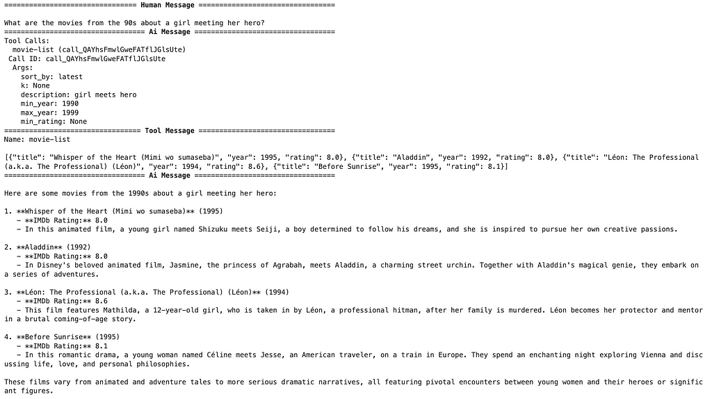
\ This time, additional arguments were used to filter movies only from the 1990s. This example would be a typical example of metadata filtering using the pre-filtering approach. The generated Cypher statement first narrows down the movies by filtering on their release year. In the next part, the Cypher statement uses text embeddings and vector similarity search to find movies about a little girl meeting her hero.

\ Let’s try to count movies based on various conditions:

\

messages = [ HumanMessage( content="How many movies are from the 90s have the rating higher than 9.1?" ) ] messages = react_graph.invoke({"messages": messages}) for m in messages["messages"]: m.pretty_print()

\ Results:

\

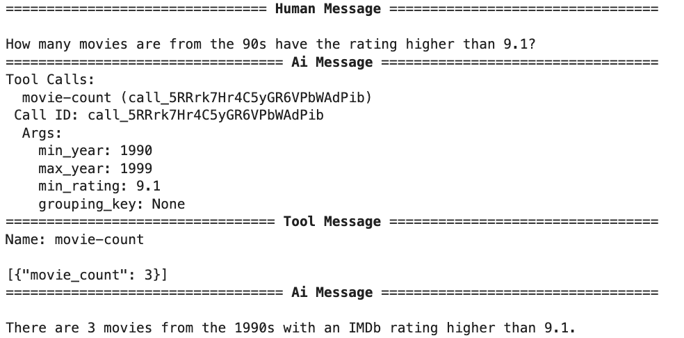
\ With a dedicated tool for counting, the complexity shifts from the LLM to the tool, leaving the LLM responsible only for populating the relevant function parameters. This separation of tasks makes the system more efficient and robust and reduces the complexity of the LLM input.

\ Since the agent can invoke multiple tools sequentially or in parallel, let’s test it with something even more complex:

\

messages = [ HumanMessage( content="How many were movies released per year made after the highest rated movie?" ) ] messages = react_graph.invoke({"messages": messages}) for m in messages["messages"]: m.pretty_print()

\ Results

\

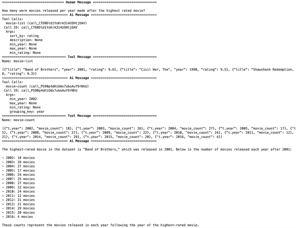
\ As mentioned, the agent can invoke multiple tools to gather all the necessary information to answer the question. In this example, it begins by listing the highest-rated movies to identify when the top-rated film was released. Once it has that data, it calls the movie count tool to gather the number of movies released after the specified year, using a grouping key as defined in the question.

Summary

While text embeddings are excellent for searching through unstructured data, they fall short when it comes to structured operations like filtering, sorting, and aggregating. These tasks require tools designed for structured data, which offer the precision and flexibility needed to handle these operations. The key takeaway is that expanding the set of tools in your system allows you to address a broader range of user queries, making your applications more robust and versatile. Combining structured data approaches and unstructured text search techniques can deliver more accurate and relevant responses, ultimately enhancing the user experience in RAG applications.

\ As always, the code is available on GitHub.

To learn more about this topic, join us at NODES 2024 on November 7, our free virtual developer conference on intelligent apps, knowledge graphs, and AI. Register Now!