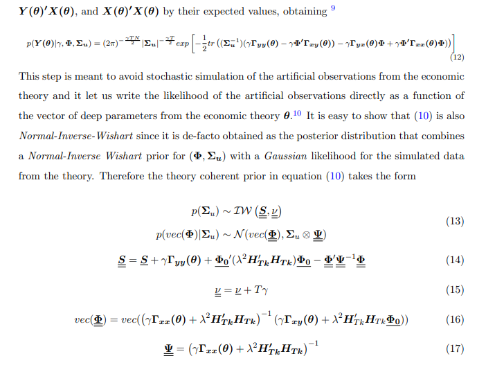
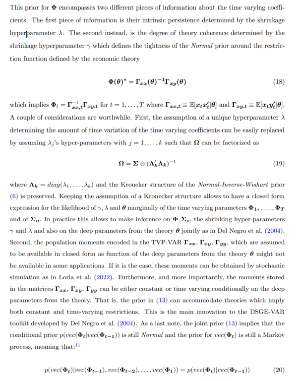
The construction of a theory coherent prior builds on the idea that an economic theory implies restrictions on the parameters of the TVP-VAR. Intuitively we can find out these restrictions by specifying a prior distribution on the deep parameters from the theory, simulating the data from the theory and then estimating a TVP-VAR on the simulated data. Imposing a prior on the deep parameters from the theory will then induce a prior on the parameters of the TVP-VAR encoding the restrictions imposed by the economic theory. Based on this idea, in this section I derive analytically a prior for a TVP-VAR which is theory coherent, in the sense that it centers the time varying coefficients on the cross equation restrictions implied by an underlying economic theory about the variables in the system.

\ Notation Before moving on, I introduce some notations conventions used in the paper. Scalars are in lowercase and normal weight. Vectors are in lowercase and in bold. Matrices are in uppercase and bold.

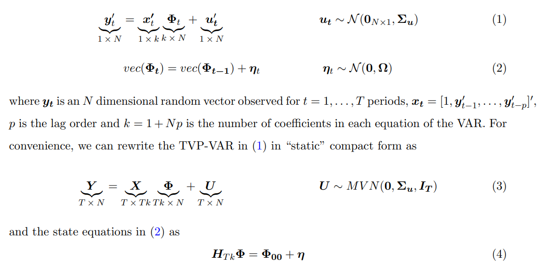
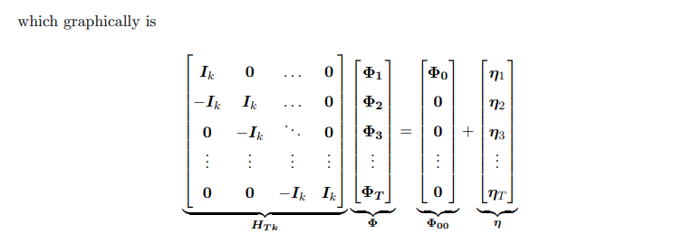
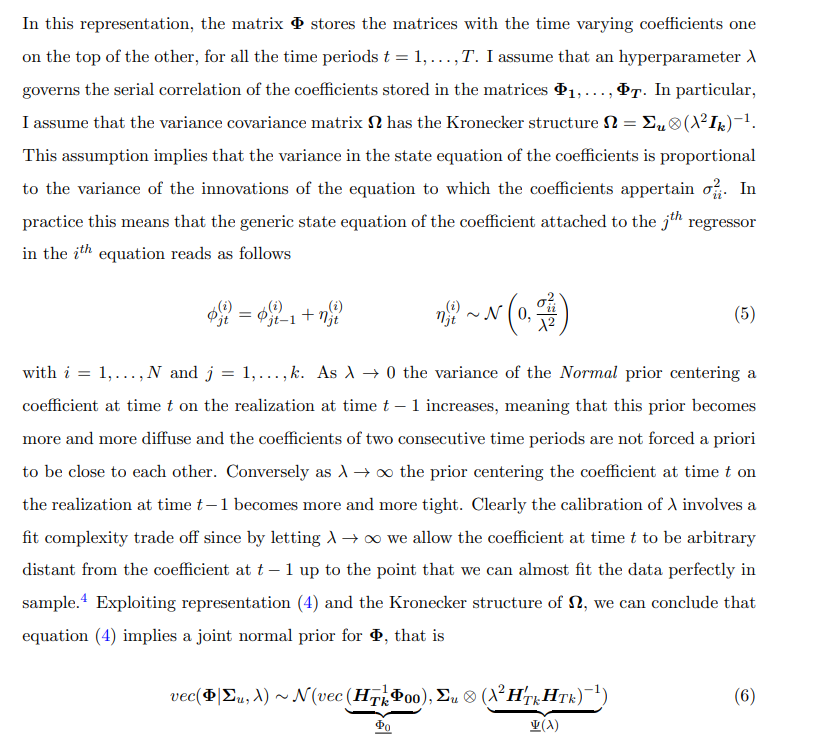
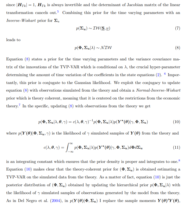
2.1 Construction of the prior

A TVP-VAR is given by:

2.2 Simulation of the prior

2.3 Conditional posterior of Φ and Σu

2.4 λ, γ and fit complexity trade off

Tuning of the optimal degree of theory coherence and the intrinsic amount of time variation of the coefficients is a delicate matter, since it clearly involves a fit-complexity trade off. As a matter of fact, very low values of both γ and λ imply a priori that the coefficients in two consecutive time periods can potentially be very different from each others and distant from the restriction functions defined by the theory.16 Intuitively, this model will fit the data very well in sample but will perform badly for forecasting out-of-sample. Indeed, decreasing γ and λ will in general increase in-sample fit of the model at the expense of out-of-sample accuracy. Based on this argument, I recommend to base the optimal choice of both the hyper-parameters on the maximization of the marginal likelihood of the model or equivalently on the maximization of the posterior of the hyper-parameters λ and γ under a flat prior for these hyper-parameters. This translates into the maximizing the one-step-ahead out-of-sample forecasting ability of the model. Indeed, the log-marginal likelihood (or Bayesian evidence) can be interpreted as the sum of the one step-ahead predictive scores, since it equivalent to the scoring rule of the form

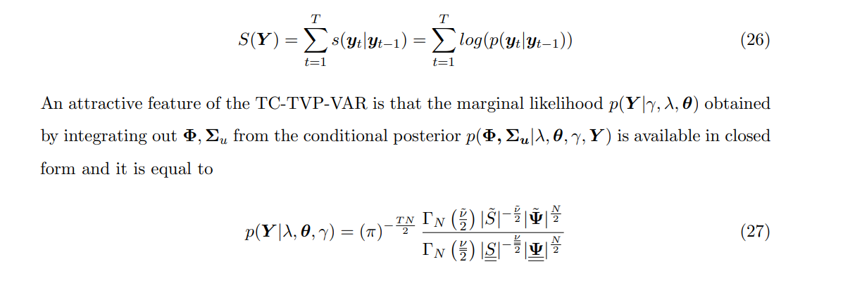
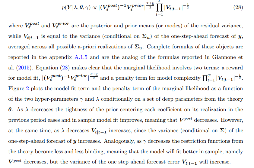
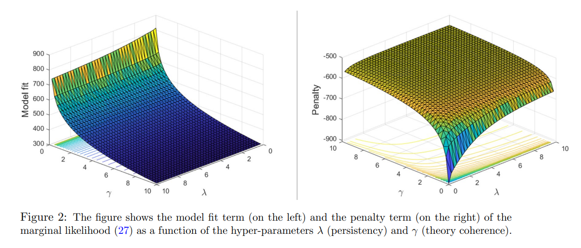
\ As a consequence, calibrating γ and λ to maximize (27) corresponds to finding γ and λ maximizing the one-step-ahead out-of-sample forecasting ability of the model. This strategy of estimating hyper-parameters by maximizing the marginal likelihood is an empirical Bayes method which has a clear frequentist interpretation. In what follows, and in particular in the estimation algorithm detailed in the next section 2.5 I will regard γ and λ as random variables and perform full posterior inference on the hyper-parameters, but analogously maximizing the posterior of the hyper-parameters will correspond to maximizing the one-step-ahead out of sample forecastability of the model. Following the same steps as in Giannone et al. (2015), we can rewrite equation (27) as

2.5 Estimation

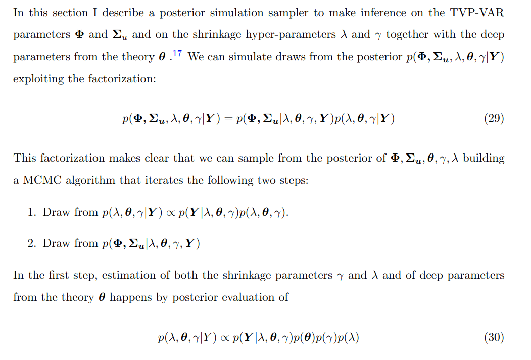
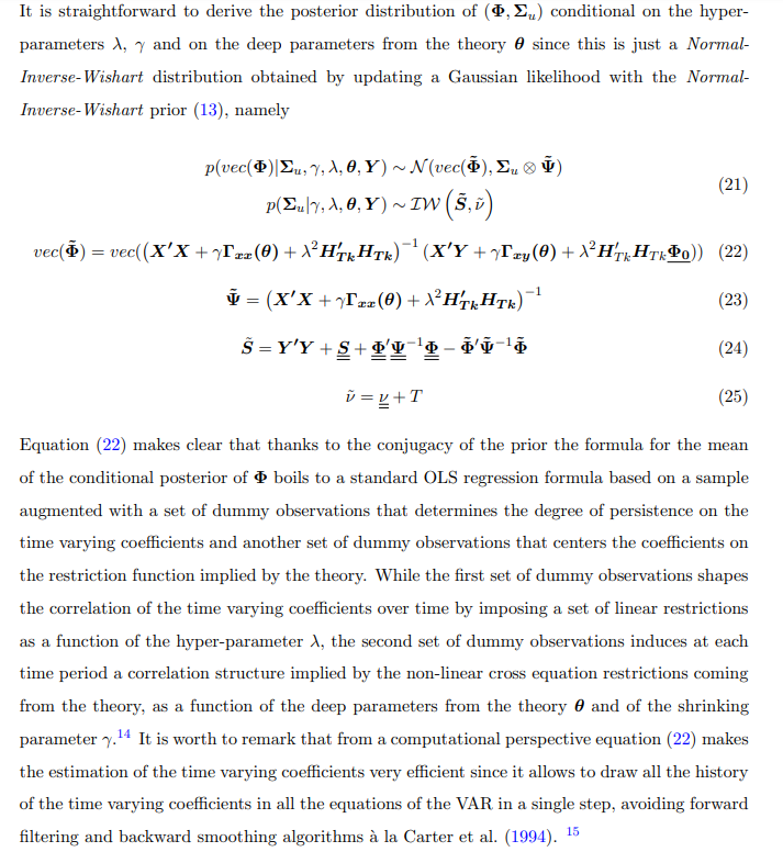
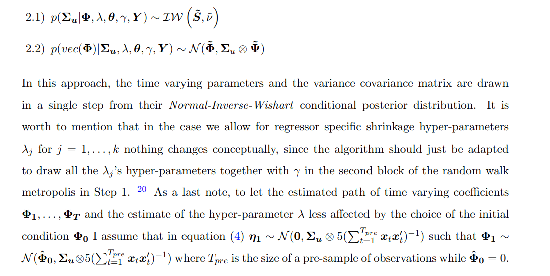
where p(γ) and p(λ) are the priors for the shrinkage hyper-parameters 18 while p(θ) is the prior of the deep parameters from the theory. Hence, learning about the structural parameters happens implicitly by projecting the VAR estimates onto the restrictions implied by the model from the theory. More precisely, the estimates of the deep parameters minimizes the weighted discrepancy between the TVP-VAR unrestricted estimates and the restriction function (18). This approach can be thought as a Bayesian version of Smith Jr. (1993) and was pioneered by Del Negro et al. (2004). In particular, the TVP-VAR is used to summarize the statistical properties of both the observed data and the theory-simulated data and an estimate of the deep parameters from the theory is obtained by matching as close as possible TVP-VAR parameters from observed data and from the simulated data.19 To sample from p(λ, θ, γ|Y ) I consider a two blocks random walk metropolis algorithm. This is basically a Gibbs Sampler where in the first block, I draw the hyper-parameters γ and λ conditionally on θ while in the second block I draw θ conditionally on the shrinking hyper-parameters γ and λ. Step 2, instead, consists just on Monte Carlo draws from the posterior of (Σu, Φ) conditional on λ, γ and θ which is the Normal-Inverse-Wishart distribution in (21) that is: \n

:::info This paper is available on arxiv under CC 4.0 license.

:::

[4.] This point will be covered more in detail in Section 2.4.

[8.] In the appendix A.1.3 I report details on the integrating constant.

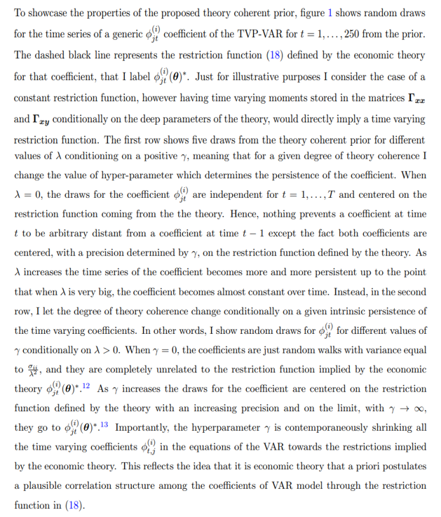
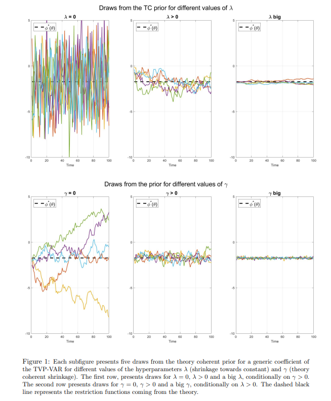
\ [12.] Note that the draws fore the time varying coefficients were initiated near the restriction functions just for visualization purposes.

\ [13.] The coefficients would have a degenerate distribution, with point mass on the restriction function.

\ [14.] In the appendix A.1.1 I show that thanks to the Kronecker structure of the prior (6) the time variation of the coefficients can be modelled by dummy observations.

\ [15.] Indeed, as in the precision sampler by Chan et al. (2009), we can draw all the latent states from t = 1, . . . , T in a single step and thanks to the Kronecker structure of the posterior, we can do it for all the N equations of the TVP-VAR jointly. More in general, the Kronecker structure (19) coupled with the precision sampler by Chan et al. (2009) can be exploited to estimate medium to large scale TVP-VARs.

\ [16.] When both γ = 0 and λ = 0 the model is left totally unrestricted, with the prior variance covariance of the coefficients being equal to infinity. Clearly, in this case there are more parameters than you can feasibly estimate with a flat prior meaning that the conditional posterior of Φ cannot be computed due to the non-invertibility of X′X (this can be seen from equation (21)).

\ [20.] Formulas for the marginal likelihood and the conditional posterior distribution of Φ and Σu can be found in the appendix A.1.6.

Feed: Hacker Noon - Medium

View: Original article

Tags: distribution trade underlying

Content Distribution