We use text-bison as the scorer and PaLM 2-L as the optimizer for all ablation studies. The tasks we evaluate are GSM8K (math reasoning) and BBH sports_understanding (non-math reasoning).

\ Meta-prompt design. The meta-prompt design is crucial in achieving good prompt optimization performance. We investigate the following core design choices:

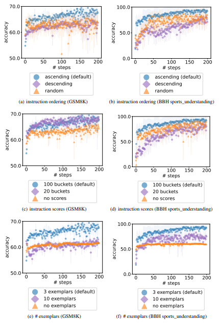
Top instructions with the highest accuracies found in prompt optimization on BBH movie_recommendation, ruin_names, and temporal_sequences.

accuracies of top instructions found for GSM8K on MultiArith and AQuA

• The order of the previous instructions. We compare the following options: (1) from lowest to highest (our default setting); (2) from highest to lowest; (3) random. Figures 7(a) and 7(b) show that the default setting achieves better final accuracies and converges faster. One hypothesis is that the optimizer LLM output is affected more by the past instructions closer to the end of the meta-prompt. This is consistent with the recency bias observed in Zhao et al. (2021), which states that LLMs are more likely to generate tokens similar to the end of the prompt.

\ • The effect of instruction scores. In terms of how to present the accuracy scores, we compare three options: (1) rounding the accuracies to integers, which is equivalent to bucketizing the accuracy scores to 100 buckets (our default setting); (2) bucketizing the accuracies to 20 buckets; (3) not showing the accuracies, only showing the instructions in the ascending order. Figures 7(c) and 7(d) show that the accuracy scores assists the optimizer LLM in better understanding the quality difference among previous instructions, and thus the optimizer LLM proposes better new instructions that are similar to the best ones in the input optimization trajectory

\ • The effect of exemplars. We compare three options: (1) showing 3 exemplars from the task (default); (2) showing 10 exemplars from the task; (3) no exemplars. Figures 7(e) and 7(f) show that presenting exemplars in the meta-prompt is critical, as it provides information on what the task looks like and helps the optimizer model phrase new instructions better. However, more exemplars do not necessarily improve the performance, as a few exemplars are usually sufficient to describe the task. In addition, including more exemplars results in a longer meta-prompt with a dominating exemplar part, which may distract the optimizer LLM from other important components like the optimization trajectory.

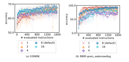
\ The number of generated instructions per step. Computing a mini-batch of gradients reduces the variance of a stochastic gradient descent procedure. Similarly, generating multiple instructions in each step improves the optimization stability with LLMs. On the other hand, to achieve better performance with a fixed budget for the number of instructions to evaluate, the number of per-step instructions should not be too large, so as to allow more optimization steps to incorporate richer information of past instructions with their accuracies. Taking both aspects into consideration, Figure 8 compares the optimization performance of sampling 1 / 2 / 4 / 8 (default) / 16 instructions in each step, showing that sampling 8 instructions at each step overall achieves the best performance

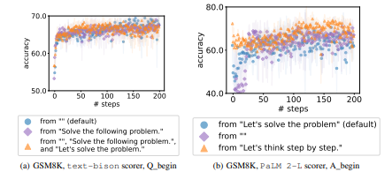
how each part of the meta-prompt matters. The dots are the averag

the initial instructions for prompt optimization. The dots are the average values across 3 optimization repetitions, and the shaded regions represent standard deviations.

Starting point. We study the effect of different initial instructions for prompt optimization. Our default setting is to start from an empty string when the scorer LLM is (instruction-tuned) text-bison, and to start from either the empty string (on BBH tasks) or “Let’s solve the problem.” (on GSM8K) with instruction position A_begin when the scorer LLM is the (pre-trained) PaLM 2-L. Figure 9(a) shows the performance of text-bison as the scorer LLM with 3 options of initial instructions: (1) the empty string; (2) “Solve the following problem.”; or (3) “Solve the following problem.” and “Let’s solve the problem.”. We observe that the accuracies do not differ much with different starting points. Interestingly, the styles of the generated instructions are also similar. For example, most of the generated instructions starting from (1) and (2) contain the phrase “solve this problem”, like “Let’s work together to solve this problem.” in Step 4 with training accuracy 64.8 from (1), and “Let’s solve the following problems using the given information.” in Step 3 with training accuracy 62.8 from (2).

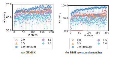
temperature of the optimizer model. The dots are the average values across 3 optimization repetitions, and the shaded regions represent standard deviations.

Figure 9(b) presents the results of of PaLM 2-L as the scorer LLM with the following options of initial instructions: (1) “Let’s solve the problem.”; (2) the empty string; or (3) “Let’s think step by step.”. We notice that the performance differs much more with different initial instructions, especially at the beginning of the optimization. Specifically, starting from (1) leads to better generated instructions than (2) in the first 30 steps, while the instructions optimized from both (1) and (2) are worse than (3) throughout. A similar observation holds when using PaLM 2-L as scorer and gpt-3.5-turbo as optimizer for BBH tasks, by comparing the results starting from the empty string (Appendix E.2) and from “Let’s solve the problem.” (Appendix E.3). Taking a closer look into the optimization process of (2), we find that although both “solve the problem” and “step by step” show up in generated instructions at Step 5, it takes the optimizer LLM more steps to get rid of worse instructions presented in the meta-prompt when starting from instructions with lower accuracies. Therefore, one direction for future work is to accelerate convergence from weaker starting points.

\ Diversity per step. We evaluate the following temperatures of the optimizer LLM: {0.0, 0.5, 1.0 (default), 1.5, 2.0}. Figure 10 shows the default temperature 1.0 achieves the best performance. Specifically, optimizations with smaller temperatures (0.0 and 0.5) lack exploration and thus creativity, and the optimizer LLM often gets stuck at the same instruction for tens of steps, resulting in flat optimization curves. On the other hand, with larger temperatures (1.5 and 2.0), the optimizer LLM more often ignores the trajectory of previous instructions presented in the meta-prompt and thus lacks exploitation, therefore the optimization curve does not have a steady upward trend.

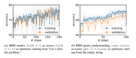
\ Comparison with one-step instruction generation. Our current iterative procedure runs for multiple steps and generates a new batch of solutions in each step. To validate the importance of leveraging the optimization trajectory for generating new prompts, we compare to a baseline that generates all instructions in a single step without entering into the optimization procedure. We compare these two approaches on GSM8K and BBH sportsunderstanding with the PaLM 2-L-IT optimizer. For GSM8K the scorer LLM is pre-trained PaLM 2-L and the initial instruction is “Let’s solve the problem”, and for BBH sportsunderstanding the scorer LLM is text-bison and the initial instruction is the empty string. The baseline generates 50 instructions in a single step, thus its meta-prompt only includes task exemplars, the initial instruction with its accuracy, and the same meta-instructions as our full meta-prompt for performing optimization. All the other hyperparameters remain the same.

\ Our results show that this one-step instruction generation performs much worse than our optimization approach. Specifically: (1) On GSM8K, the best instruction among all 50 is still “Let’s solve the problem”, with a 64.4 training accuracy and a 60.8 test accuracy. On the other hand, our approach (corresponding to Figure 1(a) in the main paper) found “Let’s do the math!” with a 78.2 training accuracy and a 76.3 test accuracy at the 5th step by generating 8 instructions at each step. (2) Similarly, on BBH sports_understanding, the best instruction among all 50 achieved a 84.0 training accuracy and 80.0 test accuracy. This is again worse than the instruction found by our approach at Step 4, which achieved a 88.0 training accuracy and a 84.5 test accuracy.

Overfitting analysis. The exemplars are splitted to 1/3 training, 1/3 validation and 1/3 test. We compute the validation accuracy every 3 steps. The training/validation dots are the average training/validation accuracies across 3 optimization repetitions, respectively, and the shaded regions represent standard deviations.

:::info This paper is available on arxiv under CC0 1.0 DEED license.

:::

Feed: Hacker Noon - Medium

View: Original article

Tags: application google options

Applications